

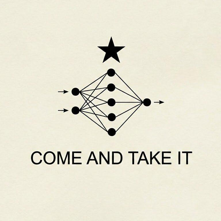
You can find no shortage of people who delight in airing their opinions about AI. For example, many have shared this meme:
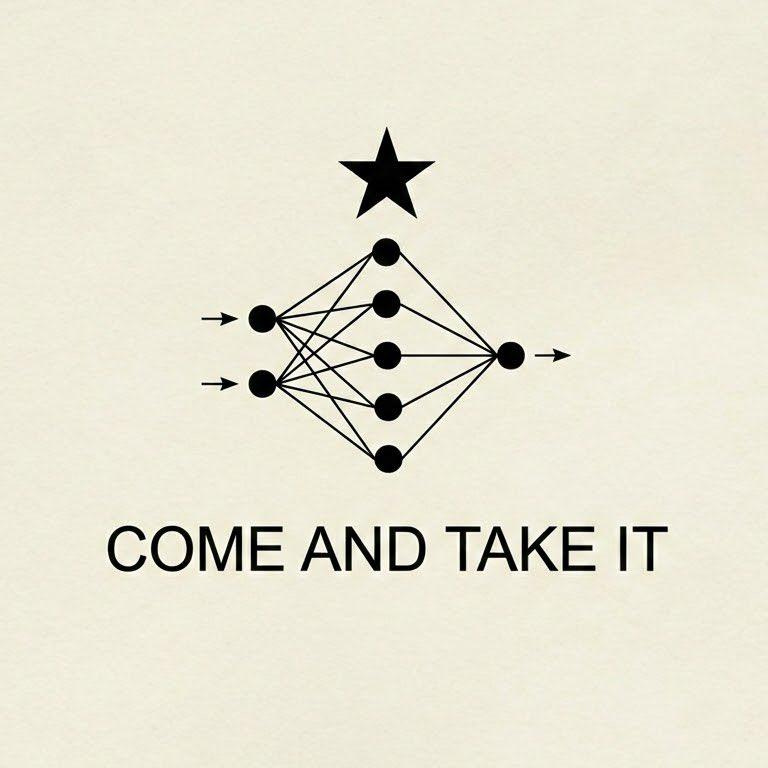
As for me, I’m going to explain how the AI in this meme works.
To quote “The Great Explainer,” American physicist Richard Feynman, “I can’t understand anything in general unless I’m carrying along in my mind a specific example and watching it go.” And that meme is a great example for understanding how AI works. You will learn how those 8 circles and numerous lines work, but our journey will start with simpler examples, beginning with a number-guessing game.
Since AI is a giant math equation, this journey cannot avoid math entirely, but the focus is on developing useful intuitions, not on manipulating math equations. (And when we do need to manipulate math equations to continue, I’ll handle that for you.)
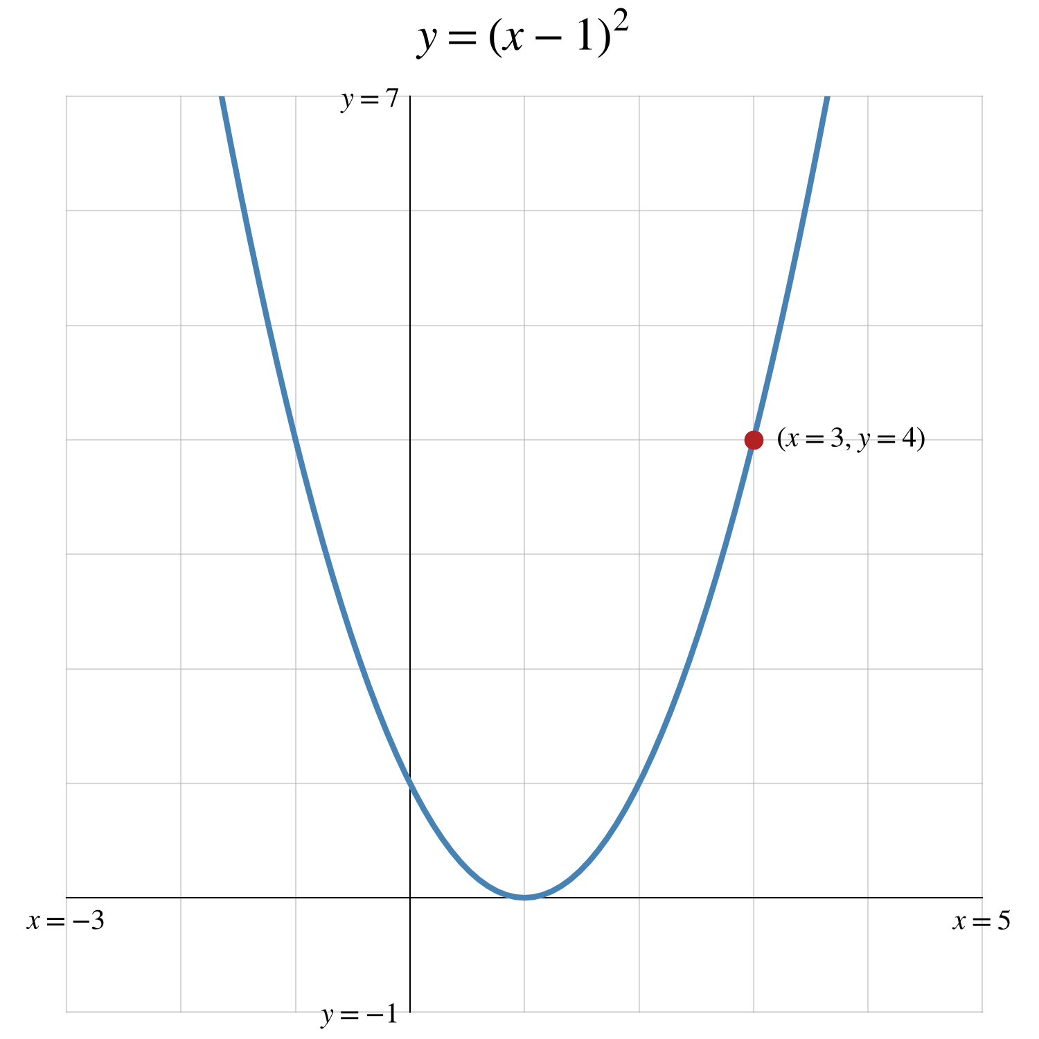
You do need to know what a function is, though. A function is just a fancy term for a math equation with an input and an output. Here’s an example:
1. How Machines Learn
Before AI, the intuition was that machines were dumb: they just mechanically follow instructions. Now that the machines can learn, though, do they become smart? To explain how machines learn, you will play a number-guessing game.
Loss
In this game, the answer (or target) is 3.5.
Your first guess (or prediction) is 5. Here is how we score that guess:
Calculate the error by subtracting the target from the prediction:
\(5 - 3.5 = 1.5\)Square the error:
\(1.5^2 = 2.25\)
This score is known as loss.
Or, more concisely, if w is your guess, and L is loss, here is the loss function:
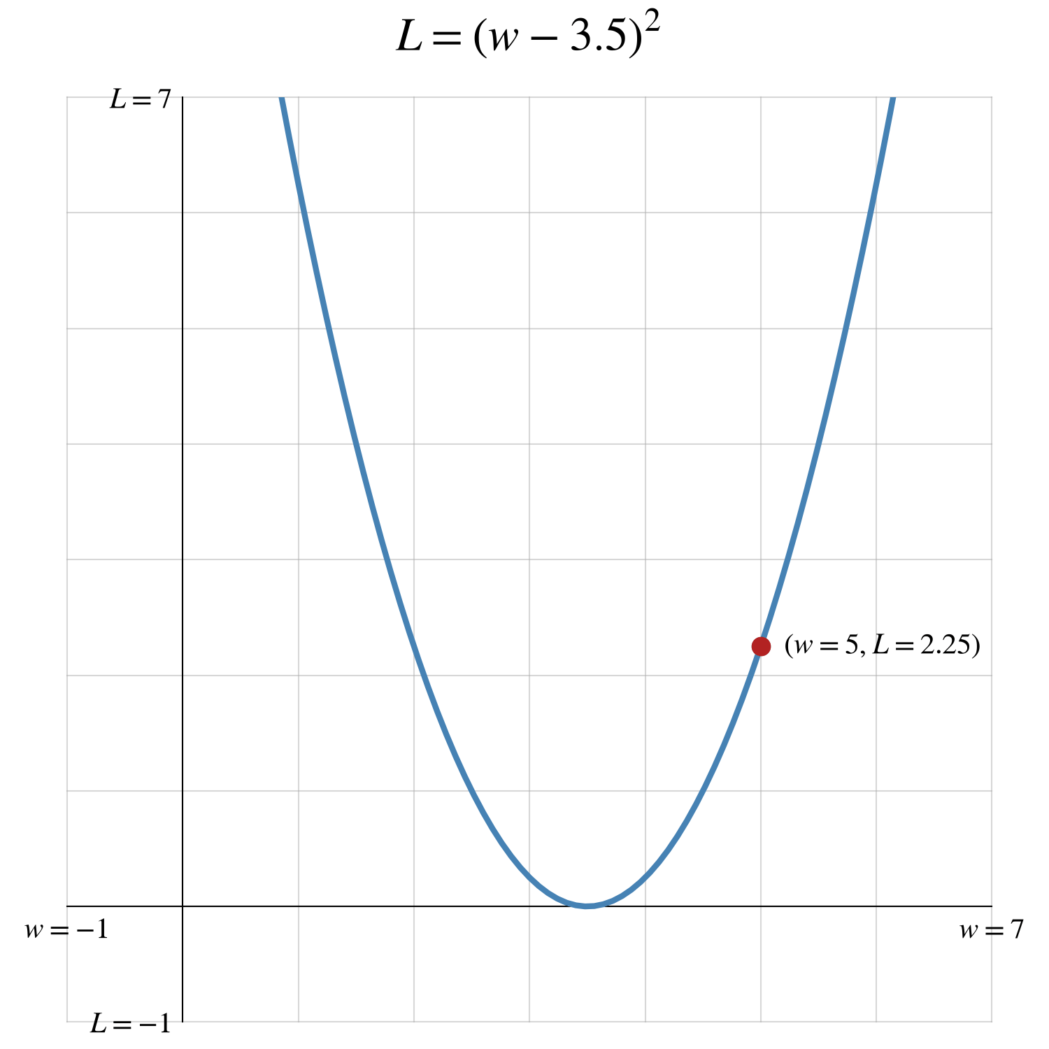
(You may be used to seeing x as the input and y as the output, but there’s no rule that you must use those two letters. And if the output is loss, it makes sense to use L.)
As you can probably figure out, the goal is to minimize loss. With that in mind, we can visualize the loss function as a hill:
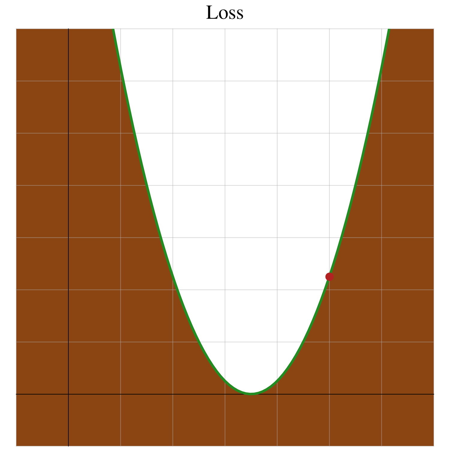
The goal is to reach the bottom of the hill.
Here, you can easily spot the bottom of the hill, but AI is a giant math equation. Navigating a giant math equation is like navigating in the darkness. So to make this example more realistic, let’s add darkness:
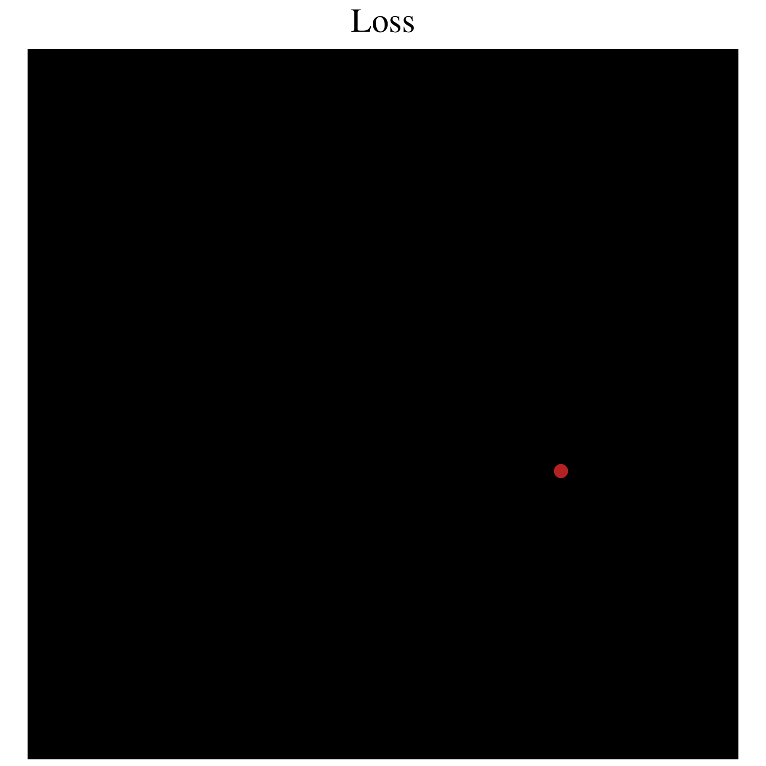
Reaching the bottom of the hill is not so easy now.
Slope
If you were standing on a hill in the dark, you could still feel the slope of the hill beneath your feet. You could tell which direction is downhill. You could tell whether the slope is steep or shallow:
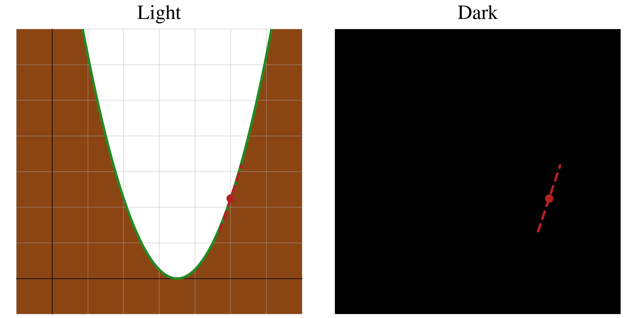
In the real world, you would take a small step downhill. In the mathematical world, though, how do you calculate the slope—much less take a small step downhill?
In short, this is what you want:
This is not a fraction; it’s a gradient. Similar to how L represents loss, ∂L/∂w represents the slope (of a function whose input is w and whose output is L).
(I can hear what the math experts are saying right about now, and frankly, I don’t care.)
To calculate the gradient, you need to use calculus. (I’ll handle the calculus for you:)
If your guess is 5, the slope (or gradient) is 3:
You now know that the gradient is 3, but what does that number mean? In short, the gradient points uphill. But how exactly does 3 point uphill? One example may not be enough, so let’s show the gradient for four guesses: 2, 3, 4, and 5.
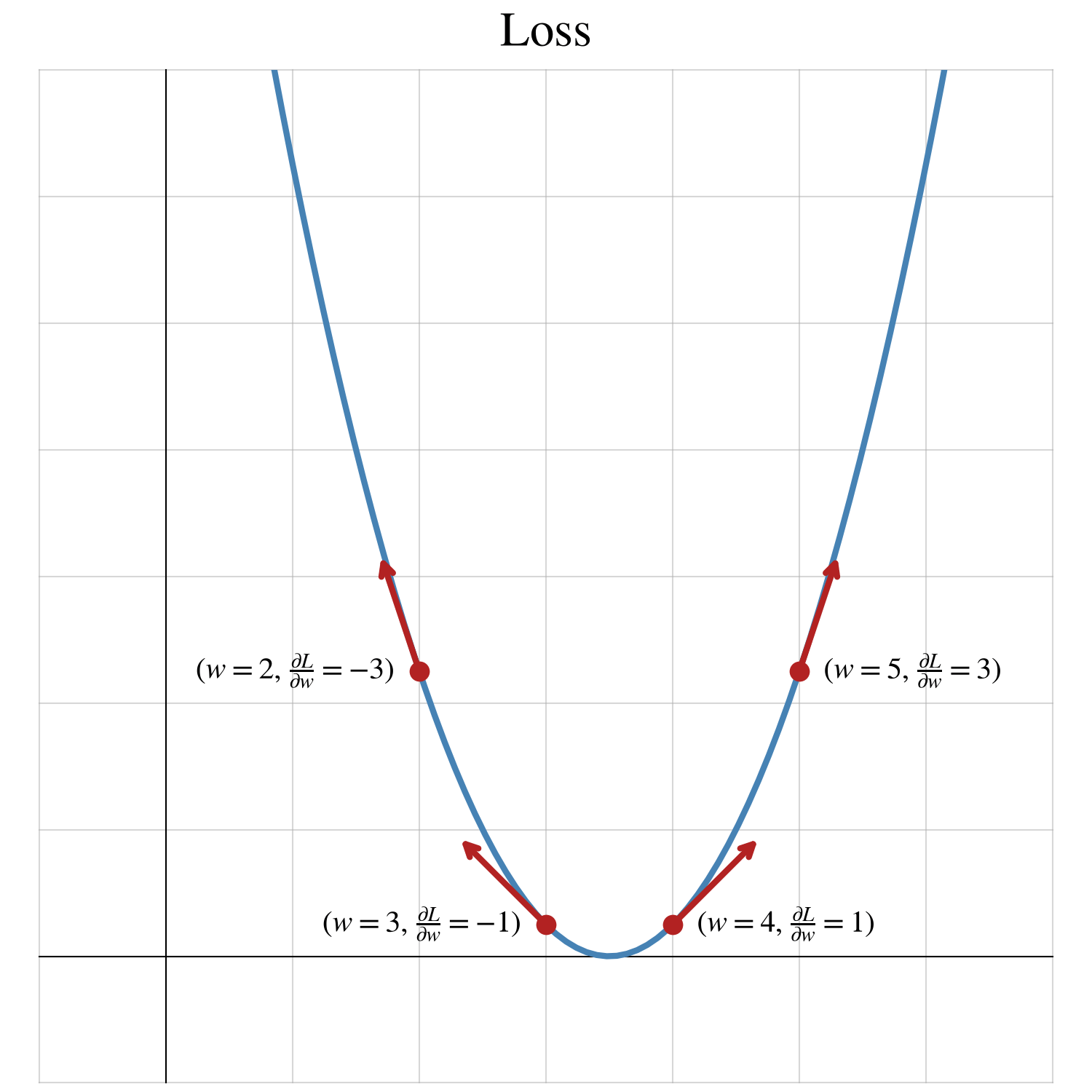
As you examine these examples, you can spot some patterns:
When the gradient is positive, you move uphill by increasing w.
When the gradient is negative, you move uphill by decreasing w.
When the gradient is larger (be it 3 or -3), the hill is steeper.
When the gradient is smaller (be it 1 or -1), the hill is shallower.
Learn
The gradient is 3, but how do you use 3 to take a small step downhill? If you moved 3 to the left (or 3 to the right), you would end up taking a very large step:
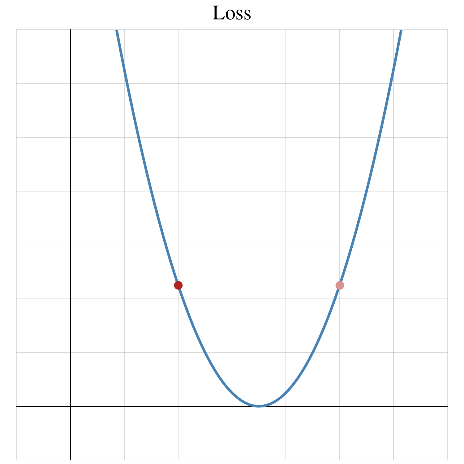
To take a small step, you first need to multiply the gradient by a small number:
The fancy term for that small number is the learning rate. (In all of the examples, the learning rate will be 0.01.)
From there, if you added 0.03 to your guess of 5, you would move uphill to 5.03:
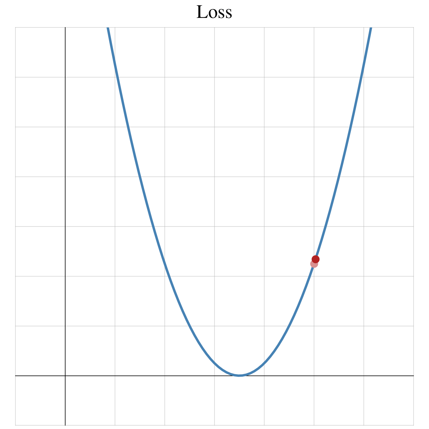
Why is that? Remember: the gradient points uphill. In this case, since the gradient is positive, you move uphill by increasing w.
To move downhill, you move in the opposite direction; subtract 0.03 from your guess:
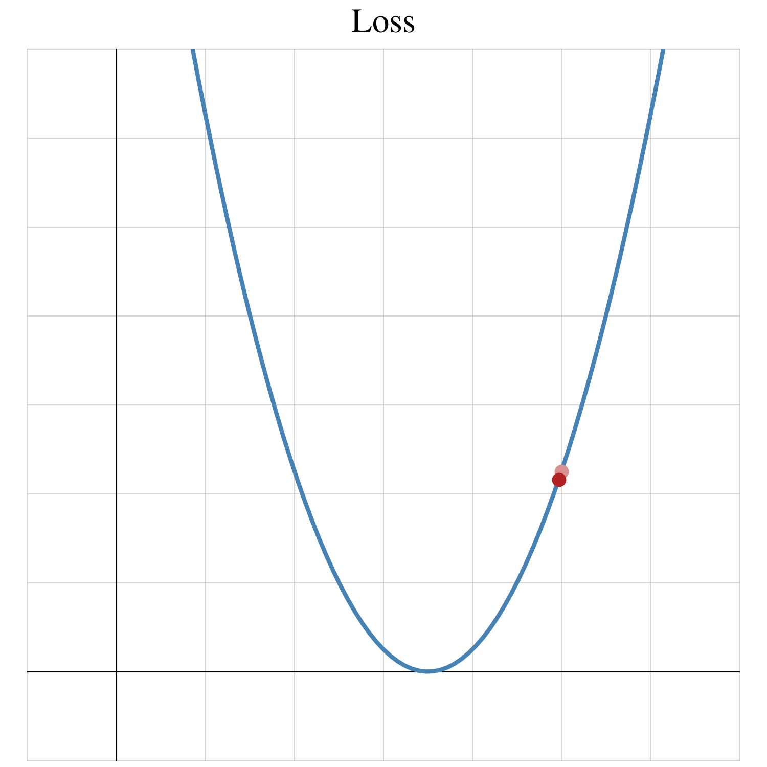
Let’s take a second small step from w = 4.97:
Calculate the gradient at your current location:
\(\frac{\partial L}{\partial w} = 2(w - 3.5) = 2(4.97 - 3.5) = 2.94\)Multiply that gradient by the learning rate:
\(0.01 \frac{\partial L}{\partial w} = 0.01 \cdot 2.94 = 0.0294\)Subtract that small value from your current location:
\(w - 0.01 \frac{\partial L}{\partial w} = 4.97 - 0.0294 = 4.9406\)
When you take 100 small steps in the dark, this short video shows what happens:
This mechanical process is called gradient descent.
Dumb Learning
Why is AI a giant math equation? If AI is a giant math equation, you can then calculate its gradient. And if you can calculate its gradient, you can then take small steps downhill using gradient descent.
With gradient descent, though, we have not left the old world of dumb machines that mechanically follow instructions. Gradient descent has no moral values. It has a mechanical goal: minimizing loss.
2. Catechizing the Bots
At times, AI can imitate human values. But if gradient descent has no moral values, then how does AI “learn” these values? Or, as James Poulos would say, “Who will catechize the bots?”
Before you opine on catechizing the bots, though, you may want to train a bot first. For the next example, you will train a bot to predict how much proline a wine has. (Proline can “impart sweetness, viscosity, and increase flavour intensity.”)
Model
Techniques exist to measure proline, but “they are either costly, laborious, or prone to severe interferences.” On top of that, you have already spent money to measure malic acid (sour and tart) and proanthocyanidins (bitter and astringent). To save money, you decide to build an AI that uses those two measurements to estimate proline.
But how exactly do you build an AI? As Cassie Kozyrkov might say, you are building a thing-labeler. In this case, the thing is wine, and the label is proline:

The inputs are two features of the thing: malic acid and proanthocyanidins.
The output is the label: proline. (The ^ [hat] symbol means that it’s a prediction.)
The fancy term for a thing-labeler is a model.
As a constructively lazy engineer, though, I don’t want to constantly type “proanthocyanidins”, so I will use some shorthand notation instead:

x₁: first feature (malic acid)
x₂: second feature (proanthocyanidins)
ŷ [y-hat]: prediction (proline)
Of course, humans have been labeling things long before AI existed. Before AI, this black box may have contained a hand-crafted math equation:

If you measure 1.77 g/L for malic acid and 2.03 g/L* for proanthocyanidins…
…this model will predict 849.5 mg/L for proline. (*The actual unit is more nuanced.)
But where did those hand-picked values (90 and 340) come from? Why do we multiply malic acid by 90? Is 90 too high or too low? That leads to an idea: instead of using hand-picked values, a machine could learn these values:

This model is now an AI model with 2 parameters (or weights): w₁ and w₂.
So how does a machine learn the values for these parameters? To train this model, you need to play another number-guessing game: guess the parameters.
Loss: One Sample
To calculate loss, you need a target and a prediction. In the number-guessing game, the target was 3.5, and the prediction was your guess. But what about this example?
This example has an extra step. You need a sample: you need to find an actual wine and measure its malic acid, proanthocyanidins, and proline. Or, if you do not want to spend money to measure proline, you can find some existing data:

This sample has 2 features and 1 target, but you need 1 prediction and 1 target. However, you have something that can turn 2 features into 1 prediction: a model.

When you feed the features into this model, though…
…you will get stuck, since the parameters are not set.
When you create an AI model, you must first initialize its parameters. Let’s use the values from the hand-crafted model as an initial guess for the parameters:

Now, when you feed the features into this model…

…it will produce a prediction.
From there, you calculate loss in a familiar way:
Calculate the error by subtracting the target [y] from the prediction [ŷ]:
\(\hat{y} - y = 849.5 - 885 = -35.5\)Square the error:
\((\hat{y} - y)^2 = (-35.5)^2 \approx 1260\)(‘≈’ means “approximately equal to.”)
Let’s add this part to the diagram:

(And from here on out, you probably will need to view these diagrams on a tablet or desktop.)
Loss: Training Data
Of course, you need more than one sample to train a model. You need a collection of samples, also known as training data:

You can repeat the same steps for each sample to obtain 3 loss values, but AI requires a single loss value. To obtain 1 loss value, let’s walk through the diagram for 3 samples:
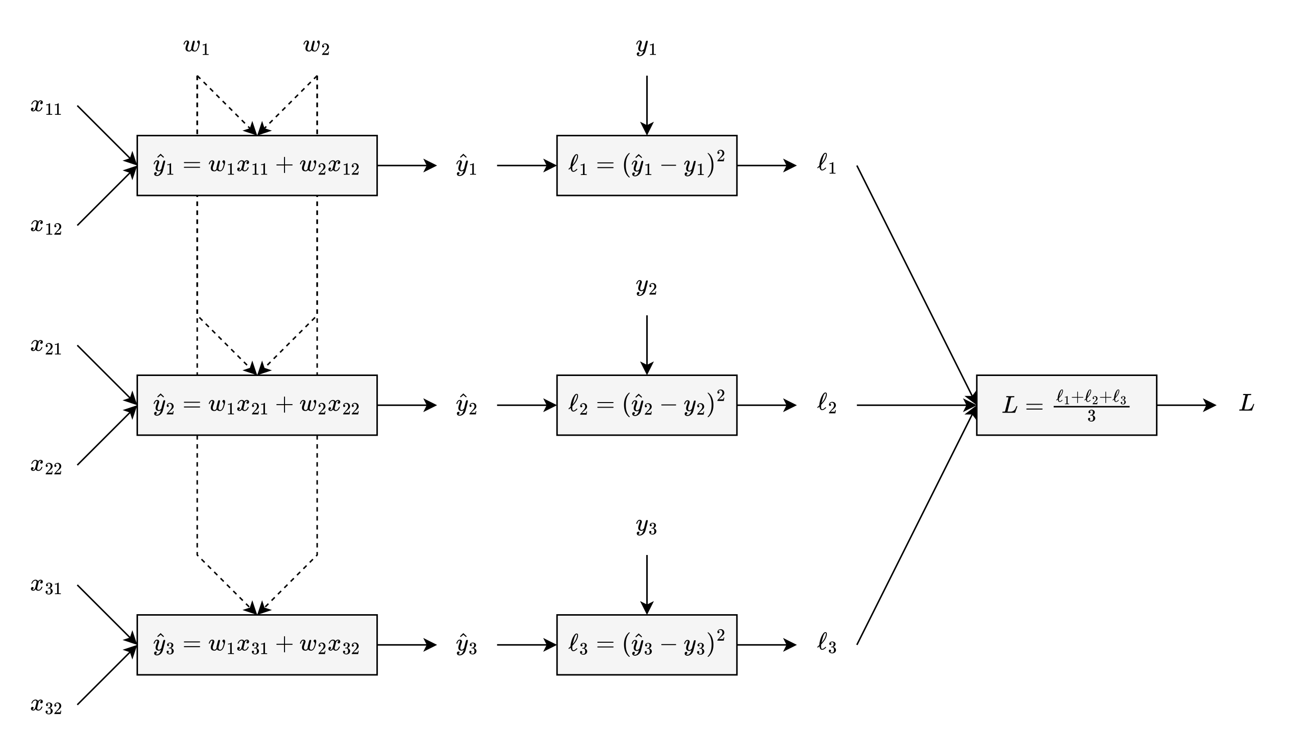
Initialize the parameters [w’s]:
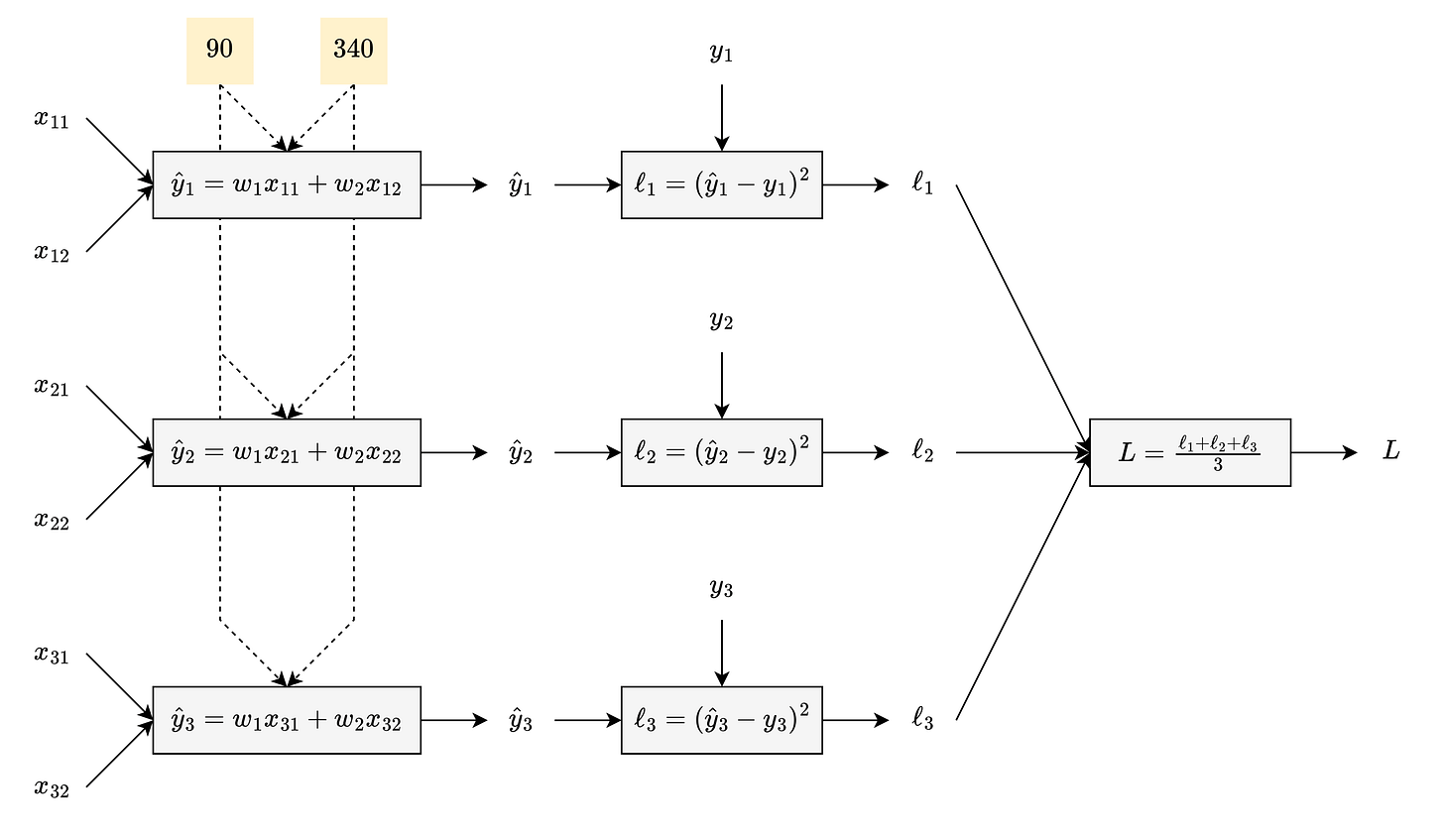
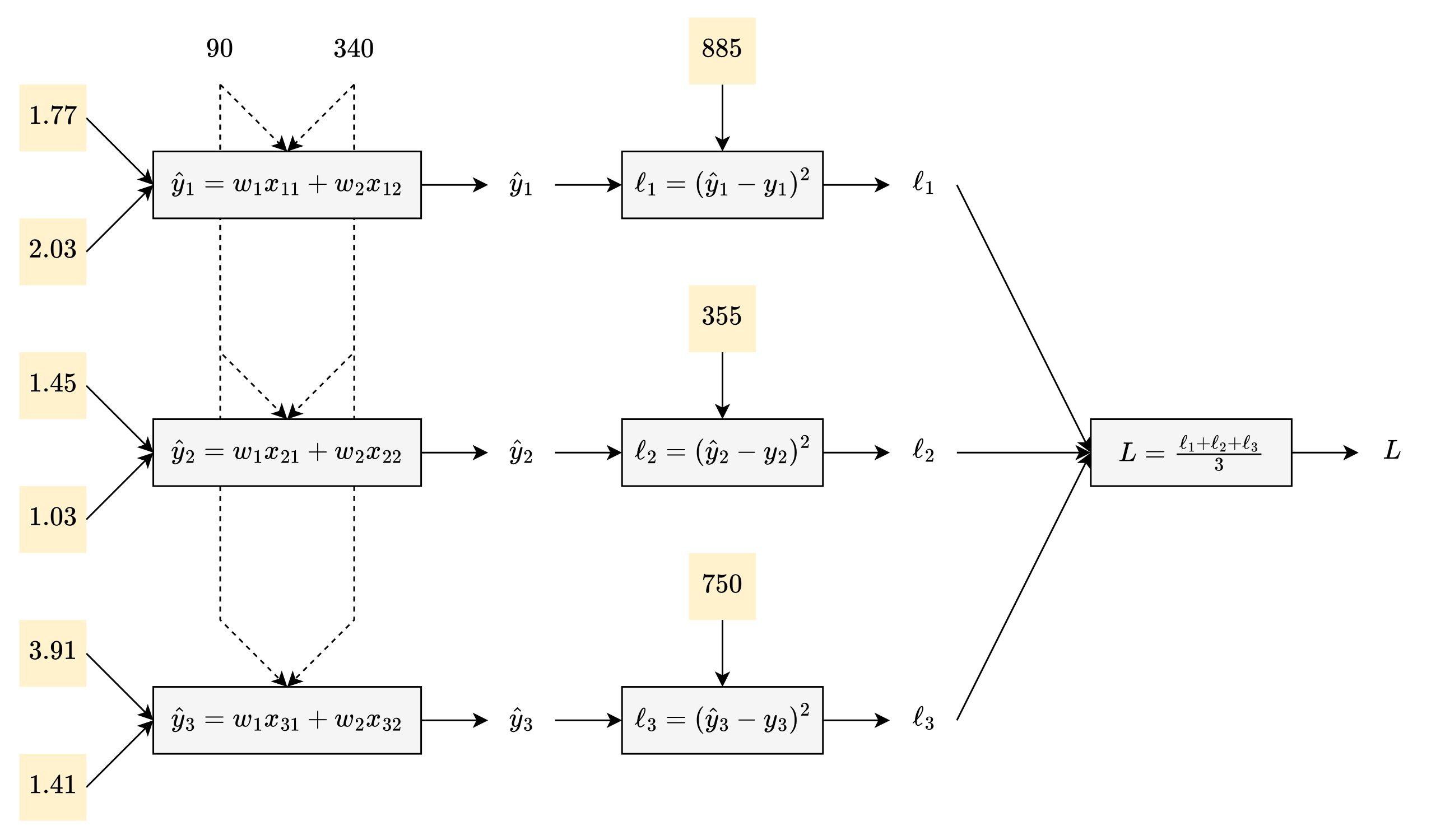
Fill in the features [x’s] and the targets [y’s] with the values from the training data:
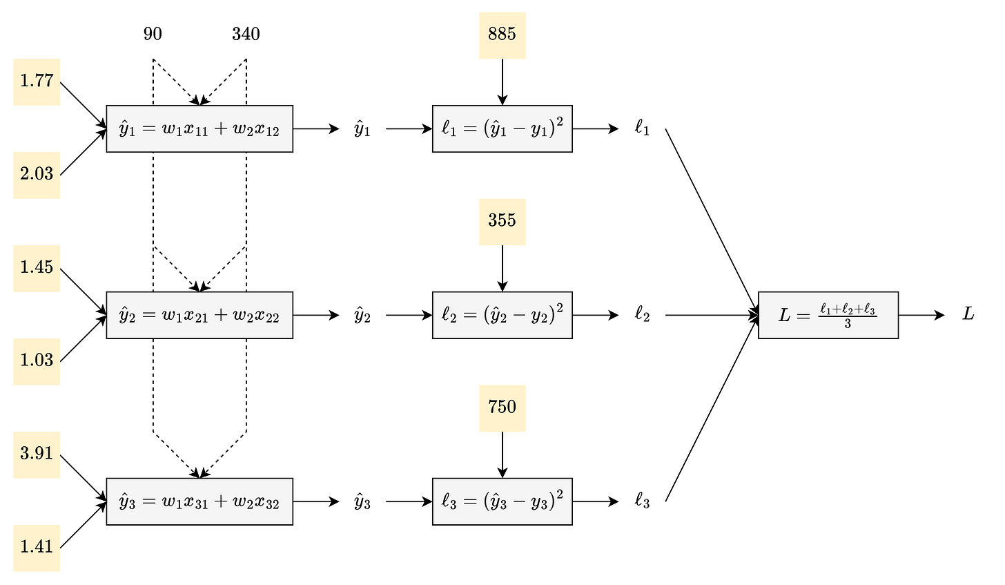
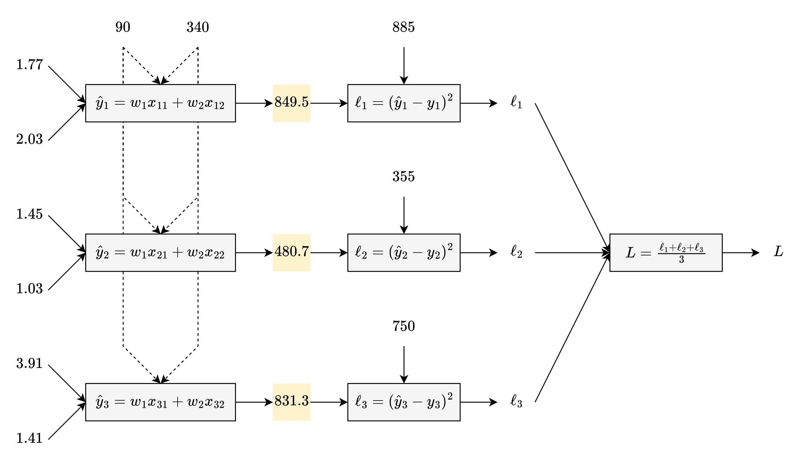
With multiple samples, x₃₂ is shorthand for third sample, second feature [1.41]. To get the predictions [ŷ’s], feed the features of each sample into the model:
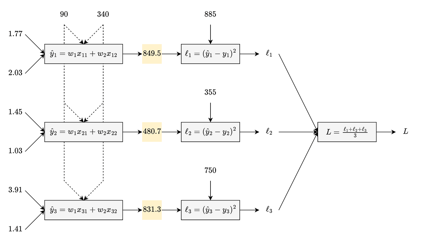
To get loss values [ℓ’s], compare each prediction to its target using squared error:
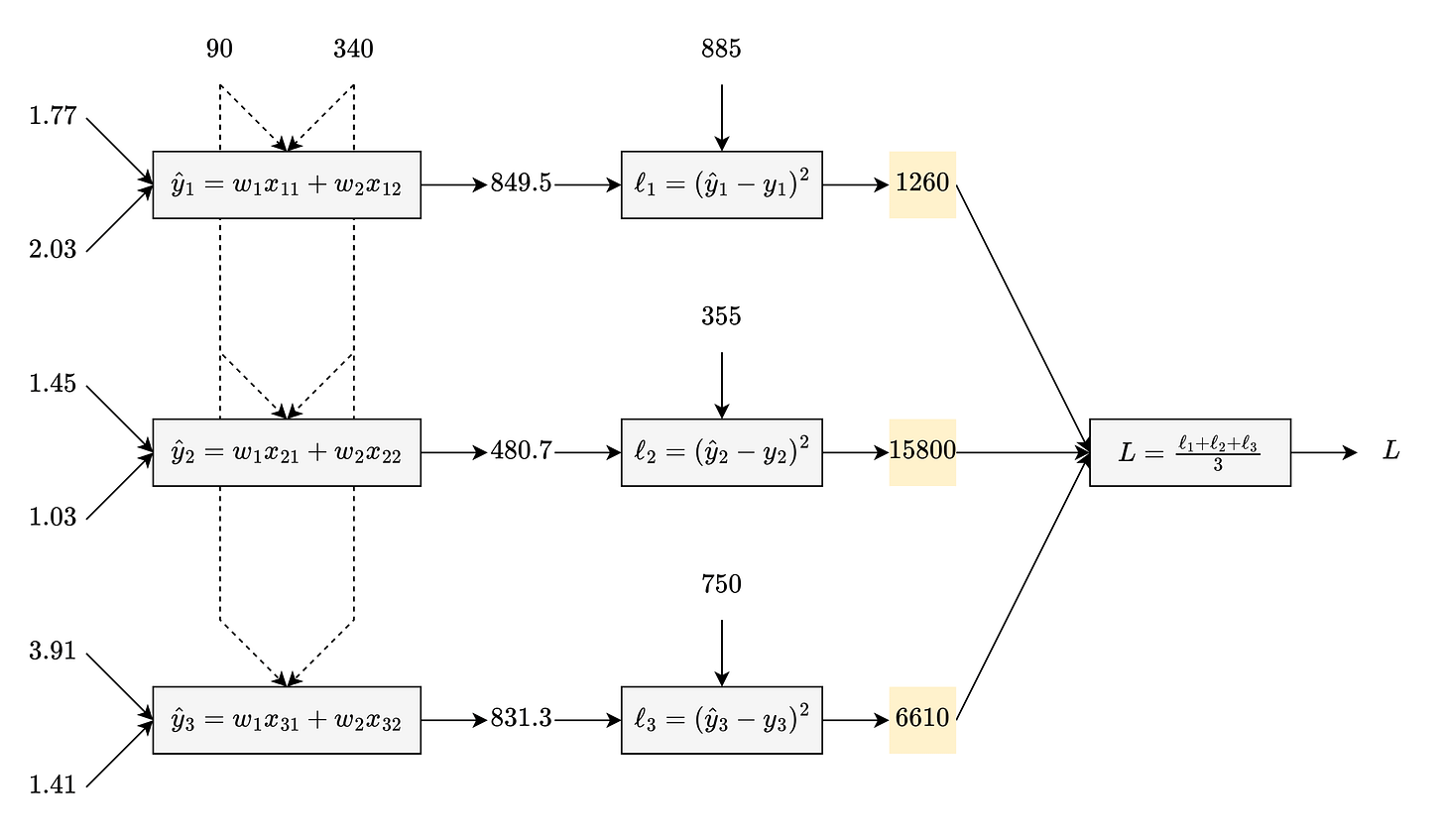
With multiple samples, ℓ represents the loss for one sample. To get 1 loss value [L], take the average (or mean) of the per-sample loss values:
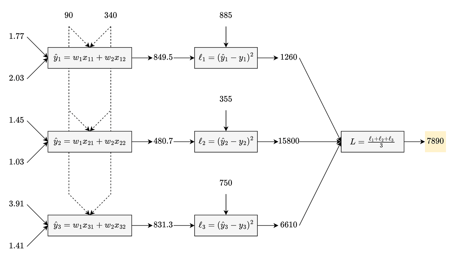
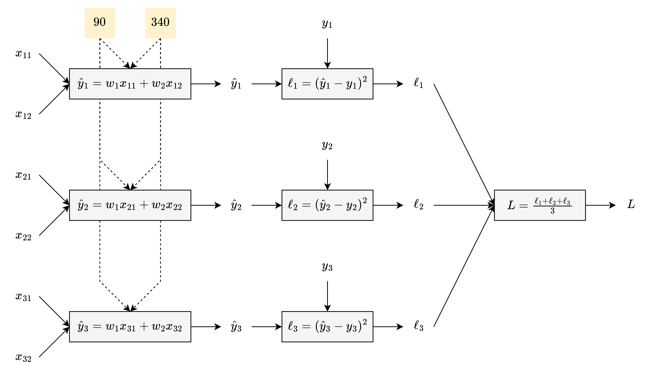
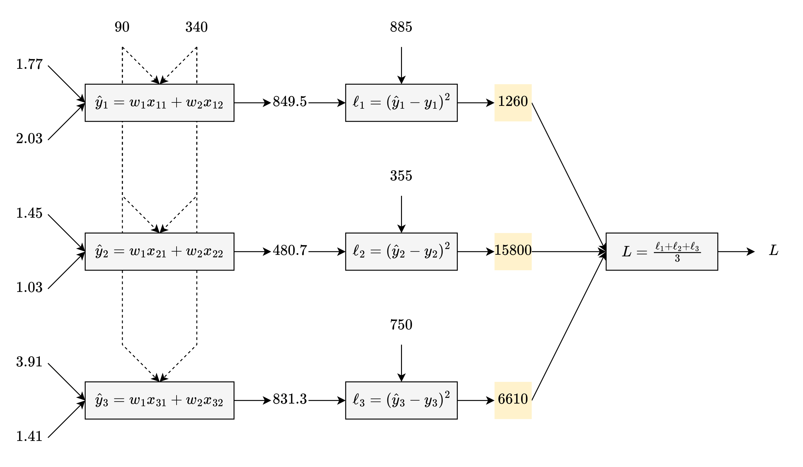
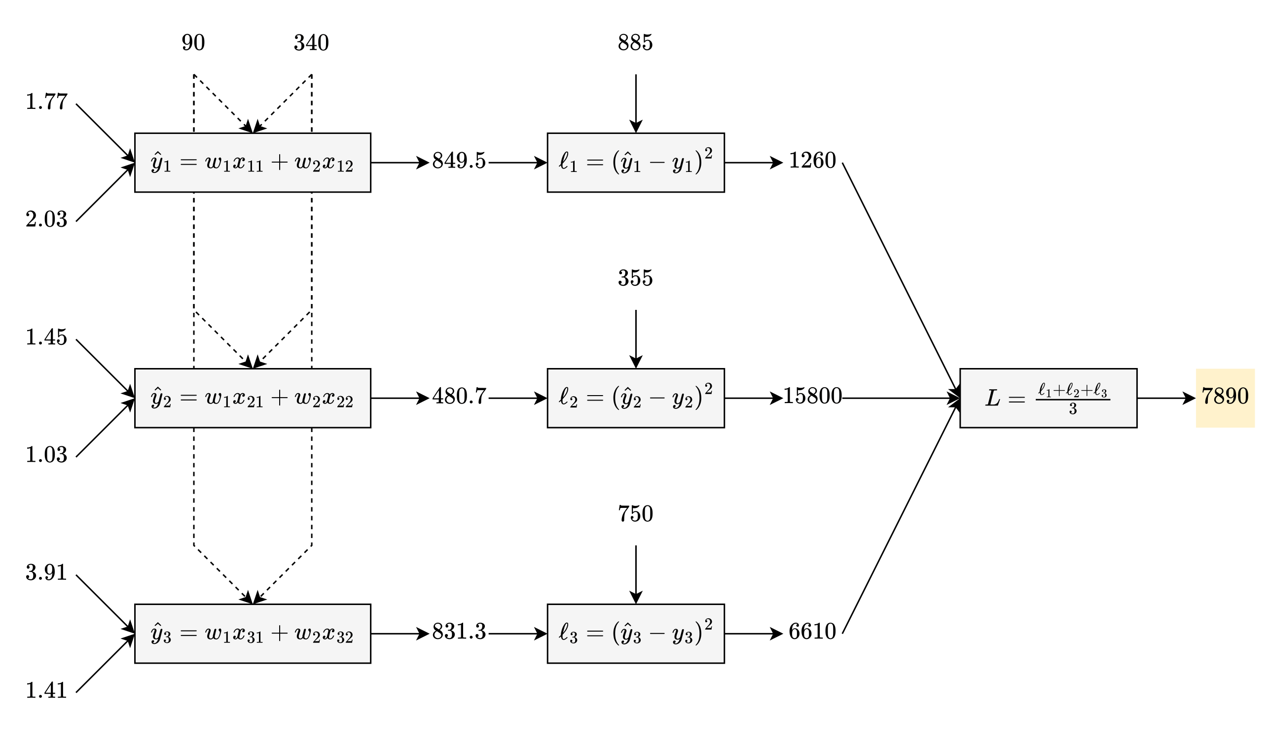
Steps 4-5 are known as mean squared error. Squared error compares 1 prediction to 1 target, but mean squared error can compare multiple predictions to multiple targets.
So what are the inputs in this diagram? If you said the features, you would be wrong…in this context. When you make a prediction with a model, that answer would be right:

The inputs are the features.
The output is the prediction.
The parameters are fixed and do not change.
When you train a model, though, you are playing a parameter-guessing game. And what are the inputs for this parameter-guessing game?
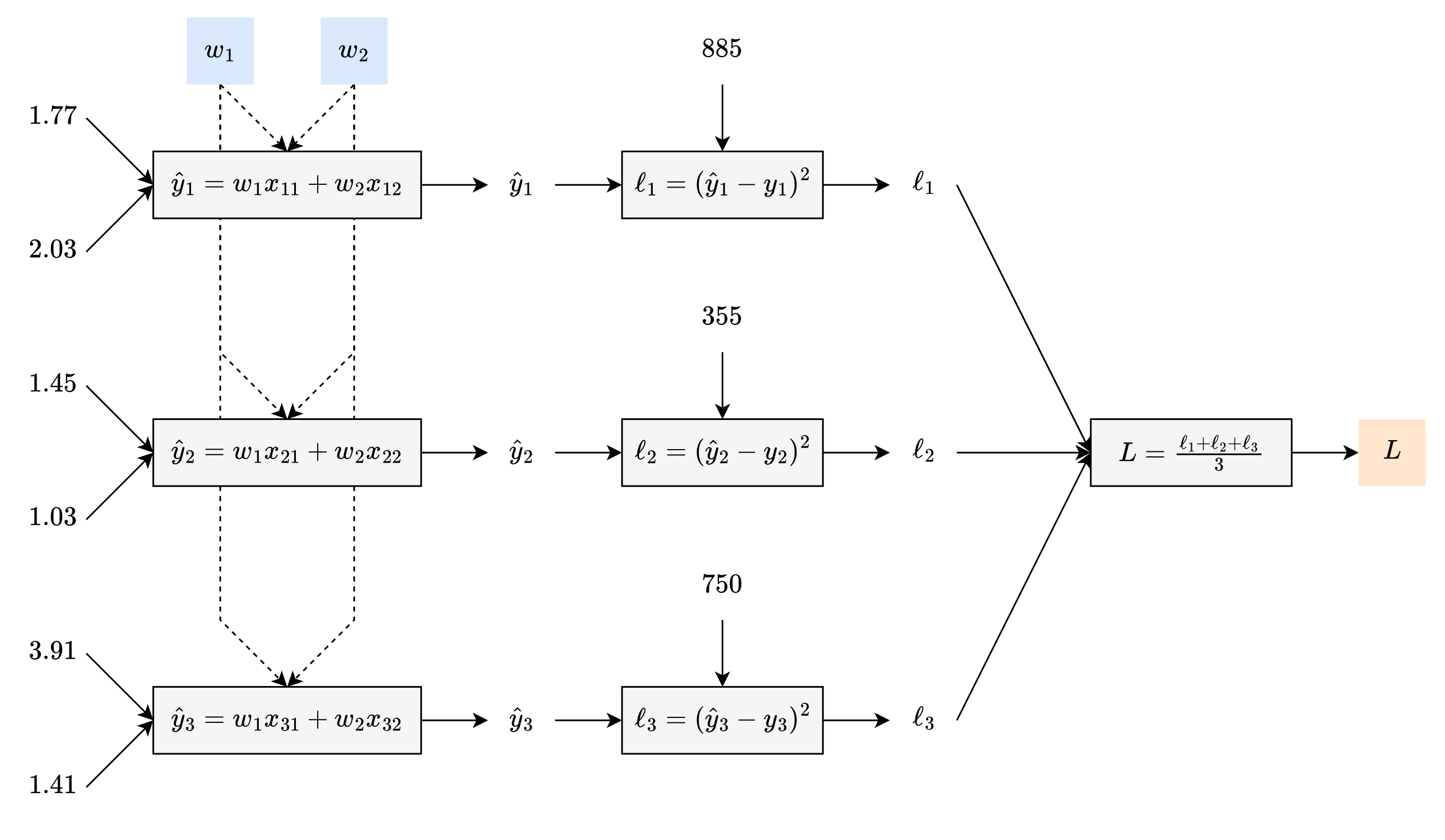
The inputs are the parameters.
The output is loss.
The features and targets are fixed by the training data.
This diagram shows the loss function—though it now has 2 inputs.
Slope
When the loss function has 2 inputs, something else changes when you visualize it:
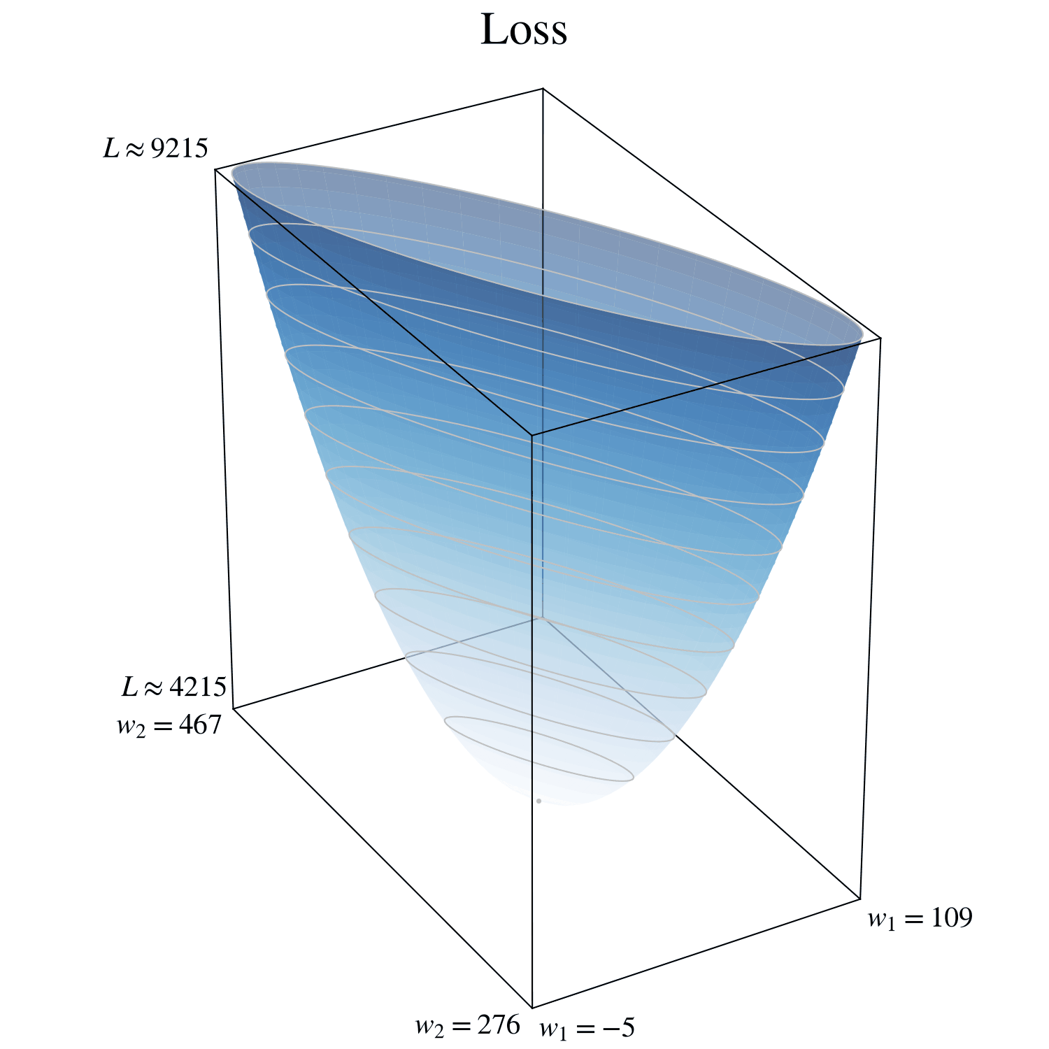
This is where I must apologize: in the number-guessing example, I lied to you…sort of. In that example, ∂L/∂w was a derivative—not a gradient.
In short, the derivative is essentially the slope of a 2D hill. But as you can clearly see, this loss function is a 3D hill; you cannot calculate the derivative of a 3D hill.
Let me ask this question, though: in the real world, if you are standing on a hill, but you can only move north or south, are you standing on a 3D hill or a 2D hill?
In the mathematical world, you are standing at (w₁ = 90, w₂ = 340). What if you fix w₂ to 340, so that you can only move by changing w₁?
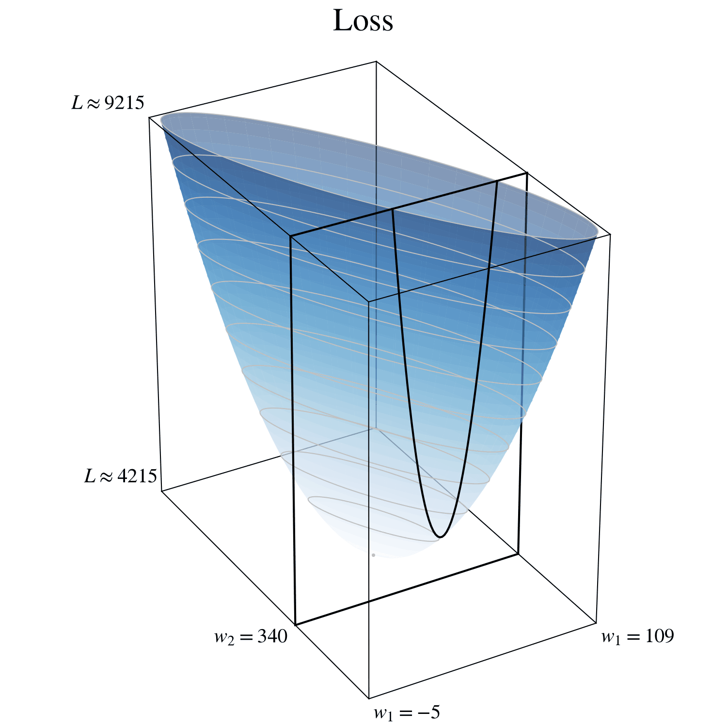
The result is a 2D hill, and the slope of that 2D hill is a derivative: ∂L/∂w₁.
And what if you fix w₁ to 90, so that you can only move by changing w₂?
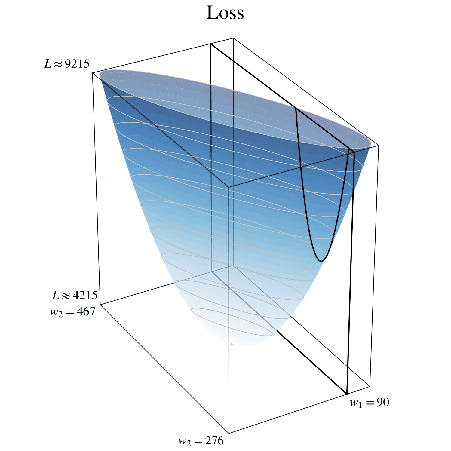
The result is another 2D hill, and the slope of that 2D hill is a derivative: ∂L/∂w₂.
In the number-guessing example, the gradient had 1 value: ∂L/∂w. In this example, the gradient has 2 values: ∂L/∂w₁ and ∂L/∂w₂. (Note to math experts: as a constructively lazy engineer, I will always use ∂. It’s harmless here.) Let’s group those values together:
(As before, I’ll handle the calculus for you:)
This equation contains ŷ’s. Is that legal? Recall how you calculated loss:
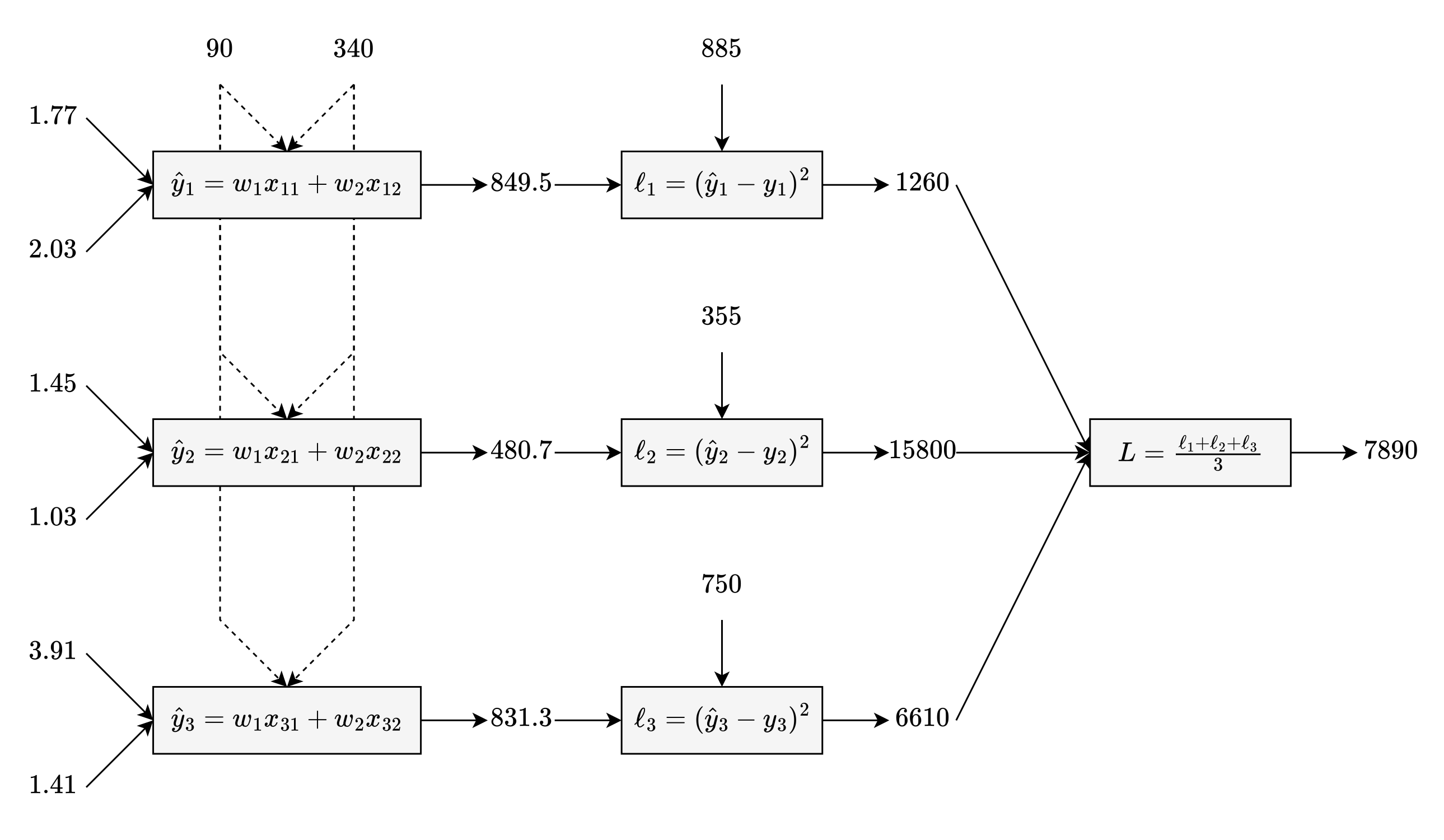
When you calculated loss, you also calculated intermediate values—including those ŷ’s. It’s perfectly legal to use those intermediate values:
Learn
When the gradient has 2 values, how do you take a single step? In the real world, if I told you to move 1 foot north and 1 foot east, you would probably take a single step northeast—not one step north and then one step east. A similar idea applies here:
∂L/∂w₁ will be used to change w₁.
∂L/∂w₂ will be used to change w₂.
So let’s take a diagonal step using gradient descent:
Calculate the loss at your current location (save all the values from this step):
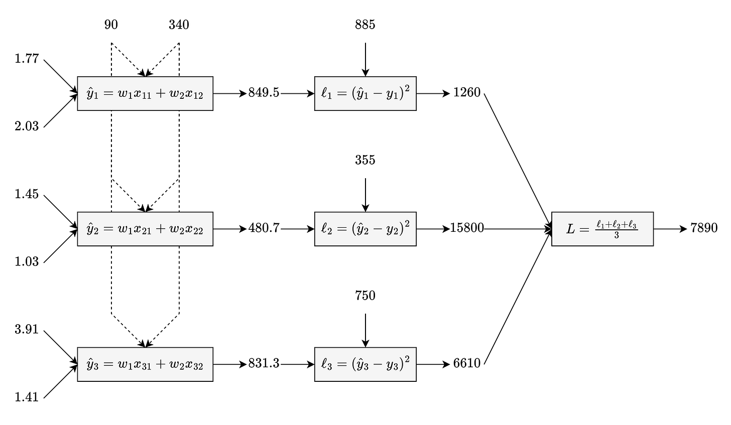
Calculate the gradient at your current location:
\(\begin{align*} \begin{bmatrix} \frac{\partial L}{\partial w_1} \\ \frac{\partial L}{\partial w_2} \end{bmatrix} &= \begin{bmatrix} \frac{3.54(\hat{y}_1 - 885) + 2.9(\hat{y}_2 - 355) + 7.82(\hat{y}_3 - 750)}{3} \\ \frac{4.06(\hat{y}_1 - 885) + 2.06(\hat{y}_2 - 355) + 2.82(\hat{y}_3 - 750)}{3} \end{bmatrix} \\ &= \begin{bmatrix} \frac{3.54(849.5 - 885) + 2.9(480.7 - 355) + 7.82(831.3 - 750)}{3} \\ \frac{4.06(849.5 - 885) + 2.06(480.7 - 355) + 2.82(831.3 - 750)}{3} \end{bmatrix} \\ &\approx \begin{bmatrix} 291.54 \\ 114.69 \end{bmatrix} \end{align*}\)Multiply that gradient by the learning rate:
\(\begin{bmatrix} 0.01 \frac{\partial L}{\partial w_1} \\ 0.01 \frac{\partial L}{\partial w_2} \end{bmatrix} \approx \begin{bmatrix} 0.01 \cdot 291.54 \\ 0.01 \cdot 114.69 \end{bmatrix} \approx \begin{bmatrix} 2.92 \\ 1.15 \end{bmatrix}\)Subtract those small values from your current location:
\(\begin{bmatrix} w_1 - 0.01 \frac{\partial L}{\partial w_1} \\ w_2 - 0.01 \frac{\partial L}{\partial w_2} \end{bmatrix} \approx \begin{bmatrix} 90 - 2.92 \\ 340 - 1.15 \end{bmatrix} \approx \begin{bmatrix} 87.08 \\ 338.85 \end{bmatrix}\)
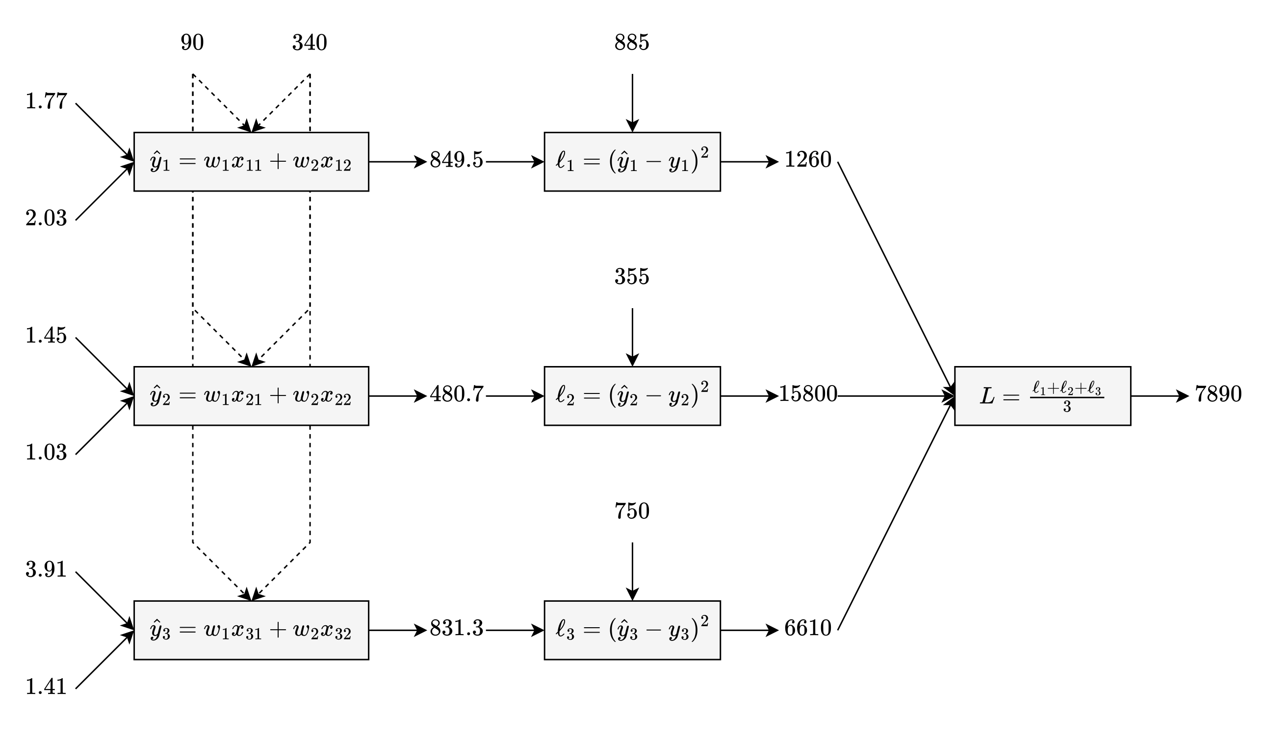
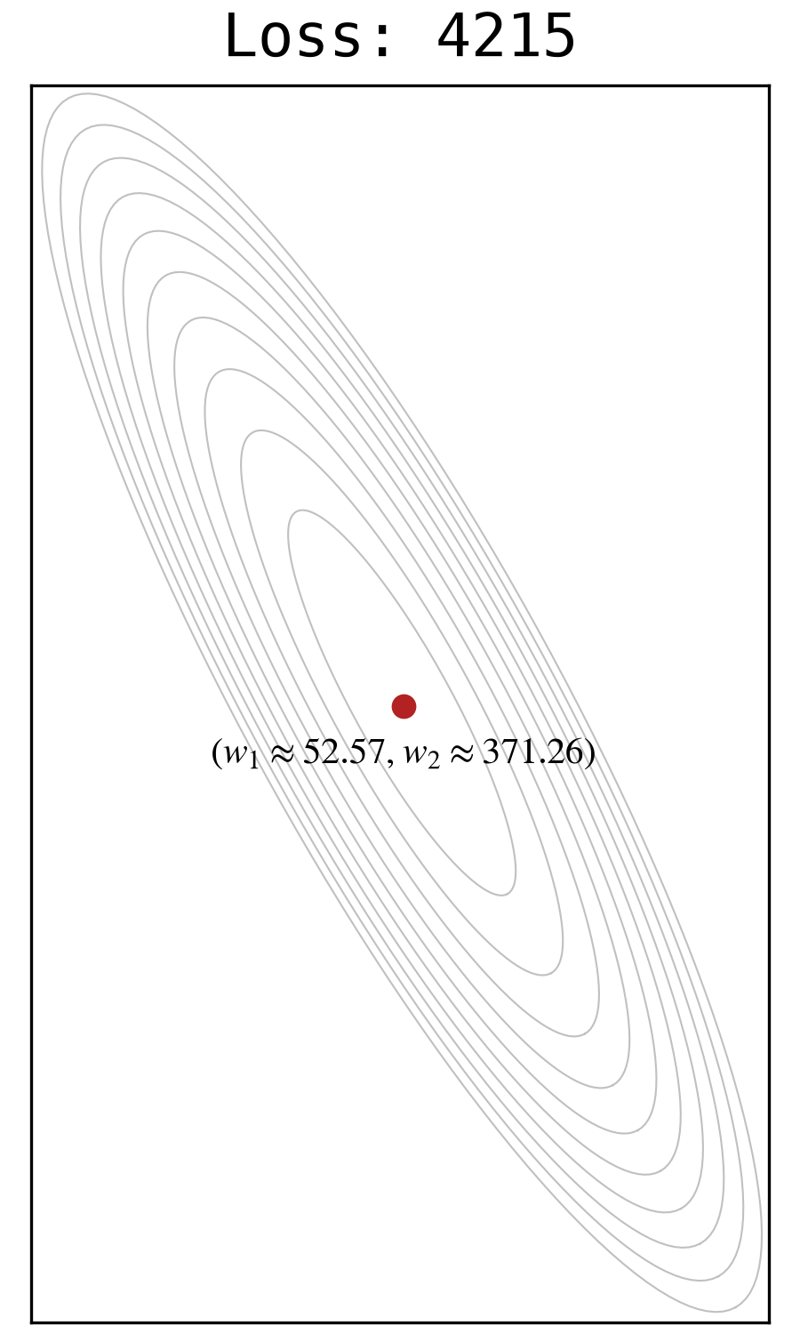
For this example, we will take 500 steps. This short video shows the first 100 steps, looking at the loss function from a top-down perspective:
Even with a 3D hill, the gradient points uphill, and gradient descent travels downhill.
After 500 steps, you end up here:
But are these new, trained parameters better than the old, hand-crafted parameters? Let’s see the model’s predictions for the training data, using both sets of parameters:

On balance, the predictions improved (although one prediction is slightly worse).
Training Data, Revisited
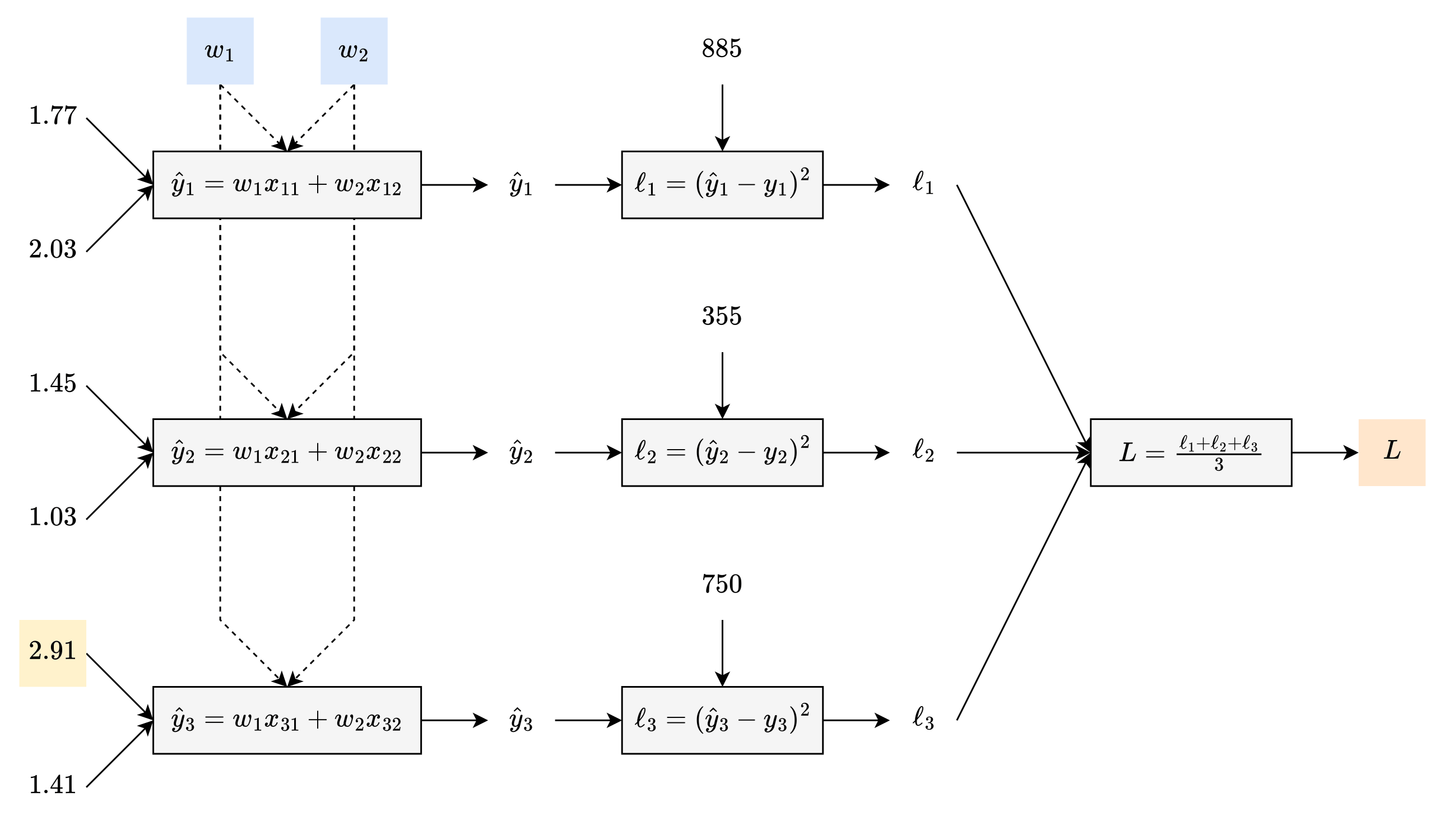
However, you just learned that the training data has a mistake: the third sample has 2.91 g/L of malic acid, not 3.91 g/L:

So what else changes when the training data changes? The loss diagram changes—which also means that the loss function changes:
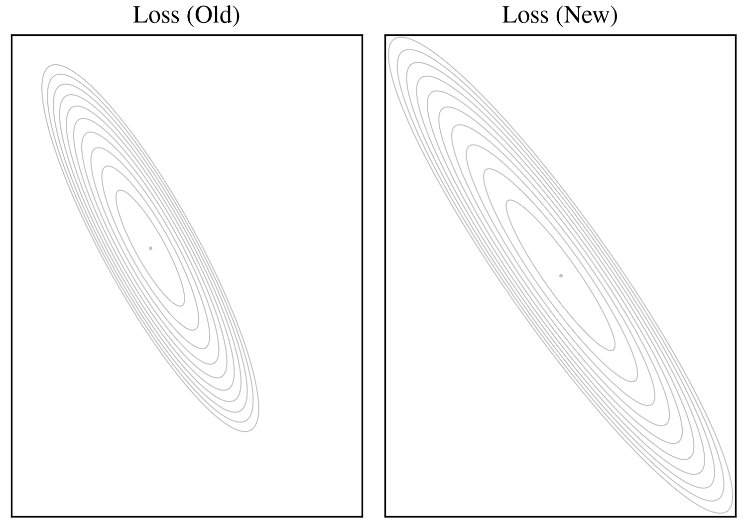
As you can see, the training data (literally) shapes the loss function.
So what else changes when the loss function changes? Gradient descent still works the same, but since it travels down a different hill, it learns different parameters:
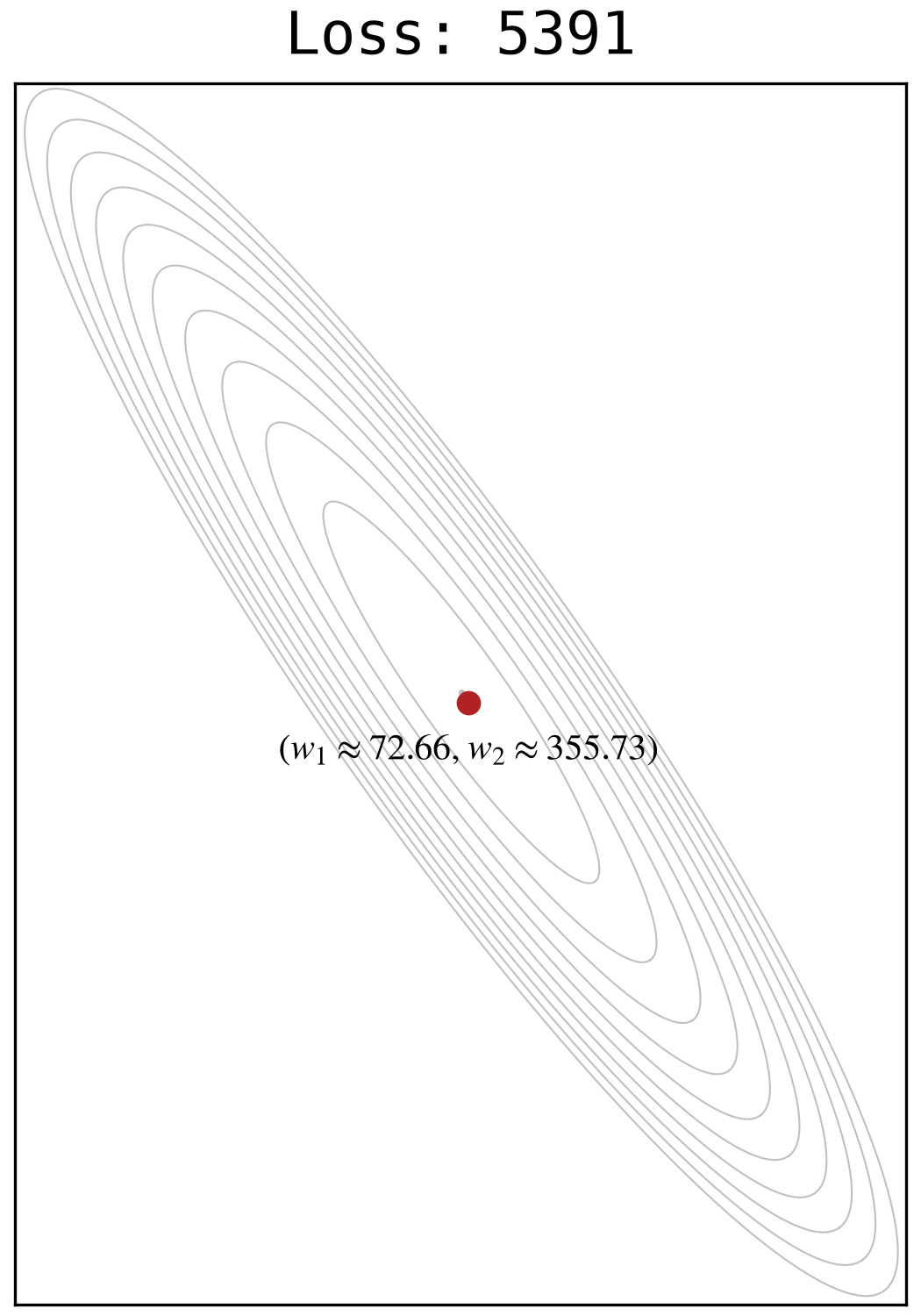
So what else changes when the parameters change? The predictions change:

Catechesis
If you change the training data, you change the parameters that the model learns. If you change the parameters, you change the model’s predictions. The training data catechizes the bot.
Now consider this model: the thing is a tweet, and the label is “hate speech” or “not hate speech.” Who will catechize this bot? The humans who curate the training data—especially the humans who label each tweet as “hate speech” or “not hate speech.”
3. The Artificial Brain
The wine model was interesting, but it hardly feels intelligent. If you’re looking for something more intelligent, that thing is a neural network, which is inspired by the human brain. And if you’re looking for an example of a neural network, here is one:
Model: Neural Network
So how does this neural network work? Let’s start by labeling the circles—and by adding two more circles:
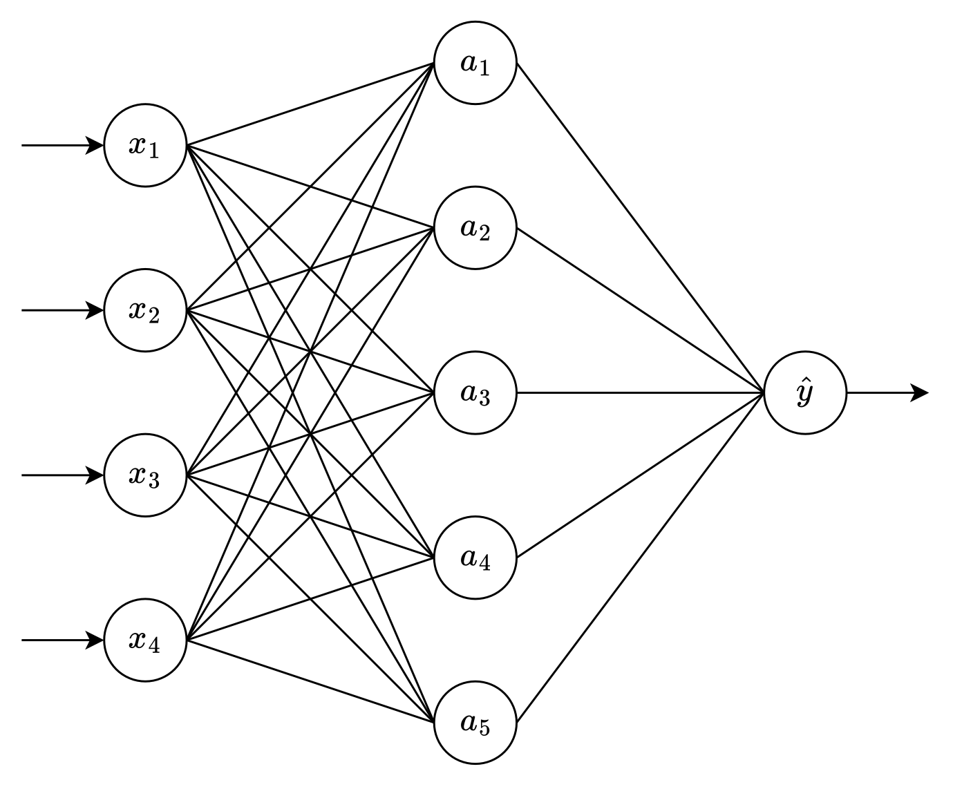
This neural network is just another thing-labeler (or model). In this case, the thing is an iris flower. As for the features of the iris flower, here is a sample:

Normally, the label would be the species: iris setosa, iris versicolor, or iris virginica.
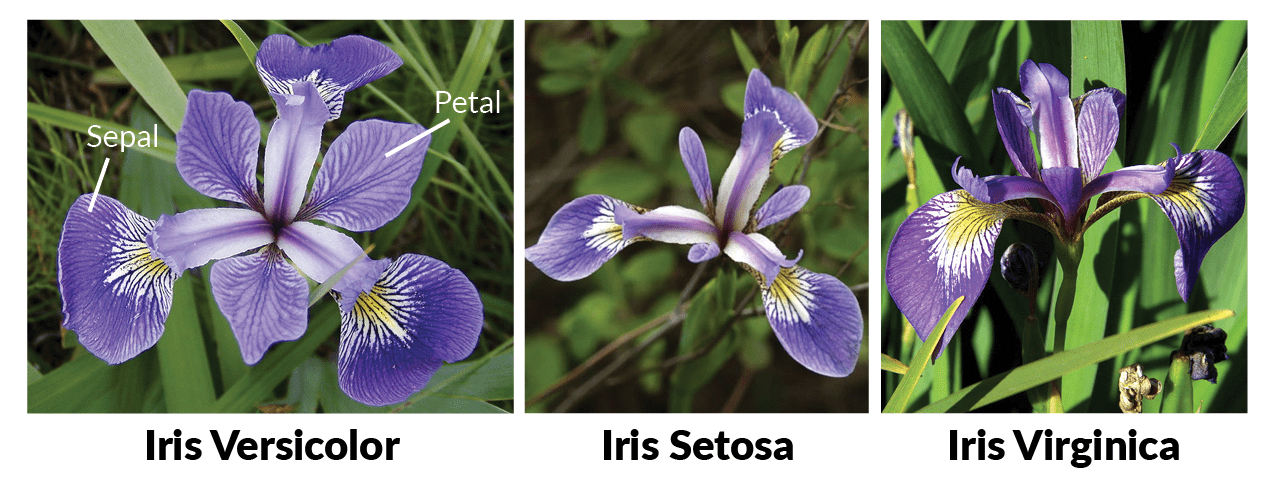
To make this example simpler, though, the label is “iris virginica”/“not iris virginica.”
As you may have noticed, this task feels different from the wine example:
When the label is a numerical quantity (such as proline), the task is a regression task.
When the label is a yes/no choice (such as “iris virginica”/“not iris virginica”), the task is a binary classification task.
Model: Input Layer
The circles are the neurons. In the human brain, a biological neuron receives signals from other neurons, and it can send a signal to other neurons.
But how do these artificial neurons work? To answer that question, take the aforementioned sample, and feed it into the neural network.
When you feed that sample into the neural network, the first stop is the input layer:
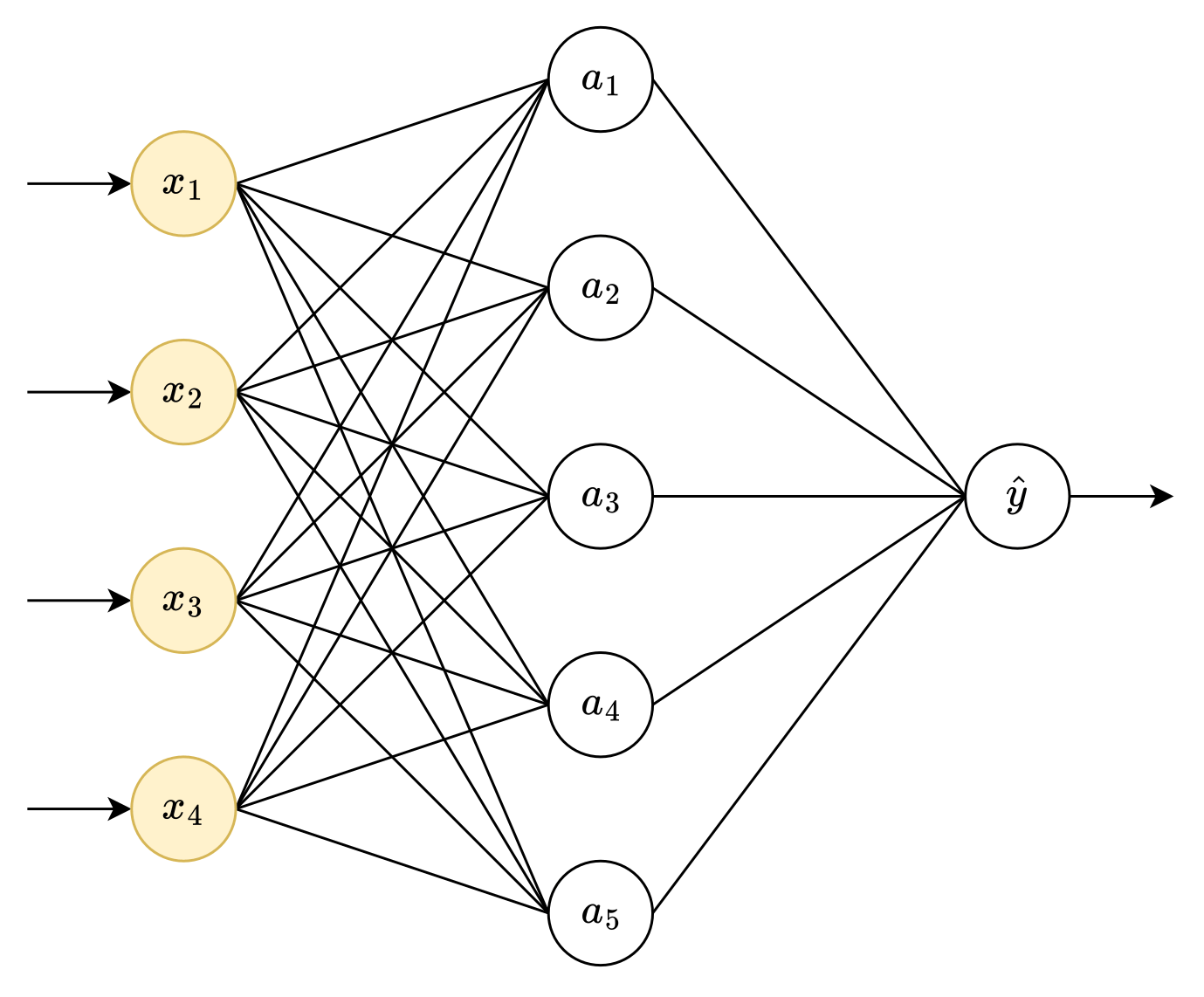
Let’s look inside this layer:
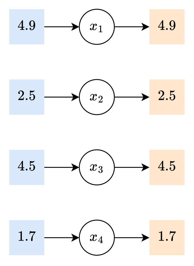
Each neuron receives the value of a feature as its input, and it also sends that same value as its output. Simple enough.
Since the input layer doesn’t really do anything, it is often excluded when counting layers and neurons. This neural network actually has 2 layers and 6 neurons.
Model: Hidden Neuron
The next stop is the first “real” layer, the hidden layer:
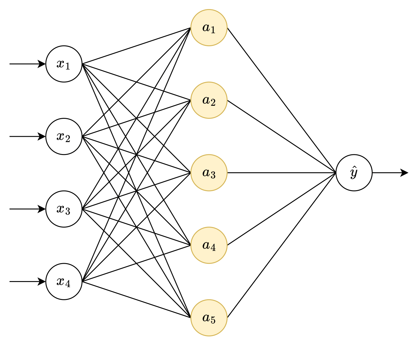
Let’s look inside this layer:
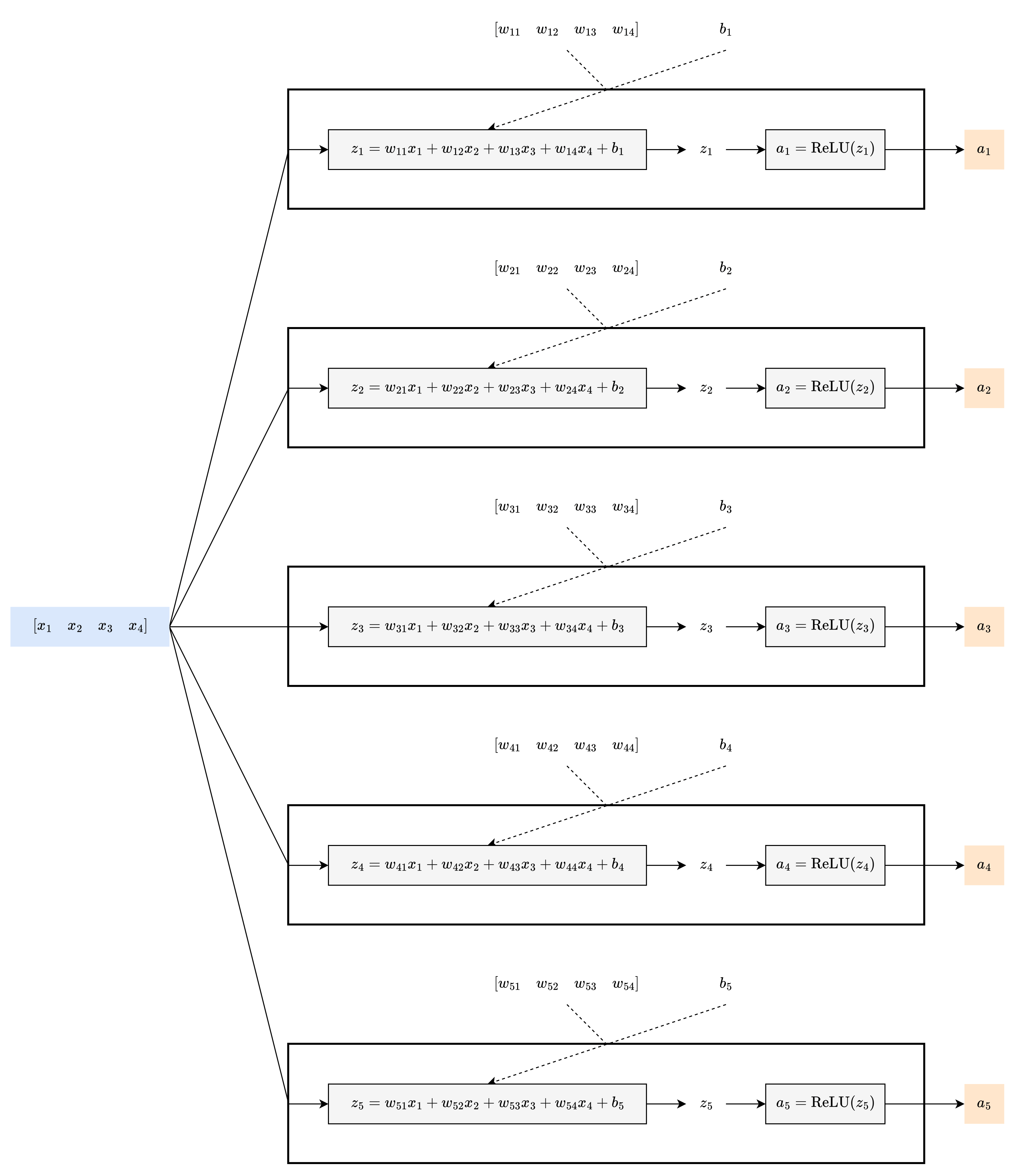
That diagram may feel a bit overwhelming. Thus, to (temporarily) simplify things, let’s start over—except this time, the hidden layer will only have one neuron.
…
The next stop is the first “real” layer, the hidden layer:
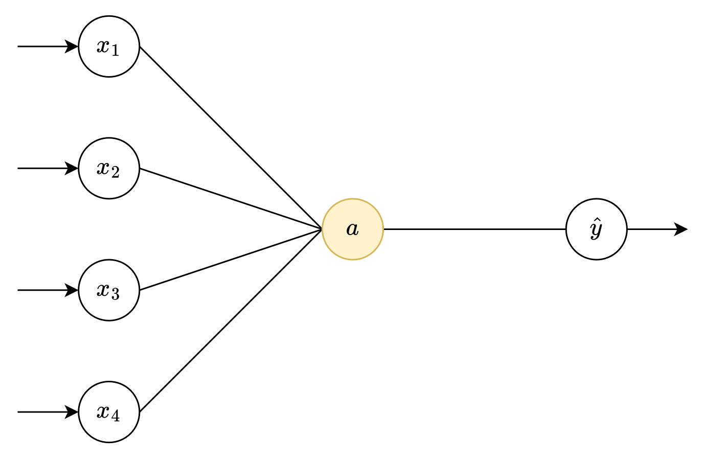
Let’s look inside this layer:
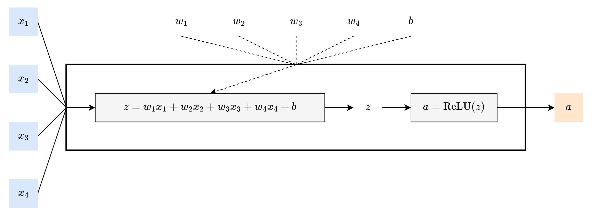
As a constructively lazy engineer, though, I prefer to draw fewer lines for 1 neuron (much less 5 neurons). So let’s group the x’s together and the w’s together:

This layer has 4 inputs and 1 output.
It also has 5 parameters. Hopefully, you remembered that the first step is to initialize the parameters. With neural networks, the convention is to use small random values:

In a biological neuron, the signals it receives from other neurons can activate that neuron. When it is activated, that neuron in turn sends a signal to other neurons.
Keep that analogy in mind as you travel through this artificial neuron. When you feed the values from the input layer into the hidden neuron…

…the first part combines those 4 values into 1 value.
As for the second part, what is ReLU? It’s easier to explain when you see it:
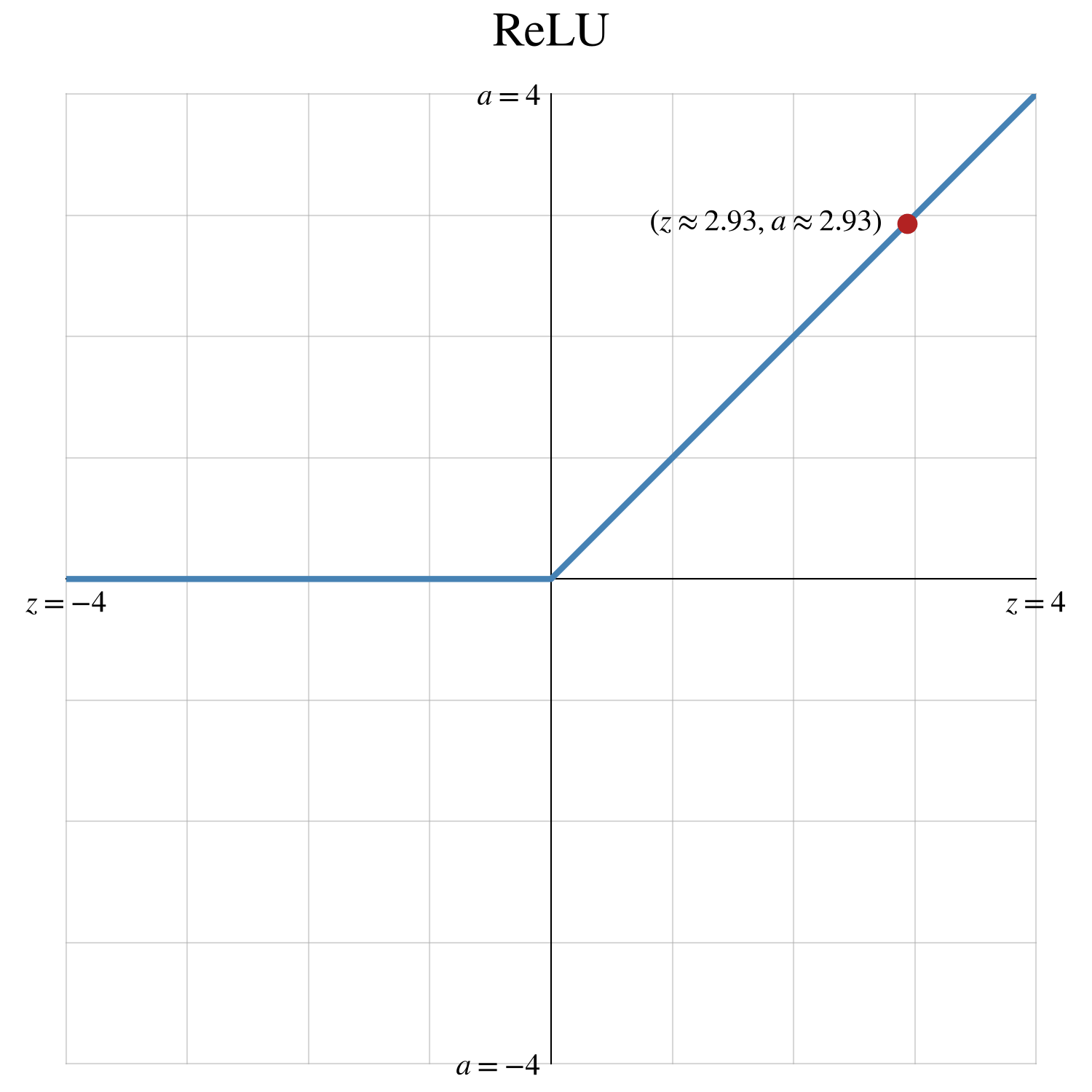
If z is positive, the neuron is activated, and the output is z.
If z is negative (or zero), the neuron is not activated, and the output is 0.
In this case, 2.93 is positive, so the neuron is activated, and the output is 2.93:

So what exactly does this neuron “learn”? Let’s revisit the first part—the part with the parameters. You vaguely understand that this part combines 4 values into 1 value, but to better understand how that combination works, let’s try some different parameters.
1. Set b to -4, and set the other parameters to 0.
b is the baseline value for the neuron. Since b is negative, this neuron starts in a non-activated state.
2. Change w₁ from 0 to 2.
Since w₁ is positive, sepal length [x₁] is a positive signal that helps activate this neuron.
3. Change w₂ from 0 to -3.
Since w₂ is negative, x₂ is a negative signal that inhibits this neuron’s activation.
This type of combination is called a linear combination. When you train this neural network, this neuron will learn how to combine its inputs into 1 value.
Model: Hidden Layer
Let’s return to a hidden layer with 5 neurons:
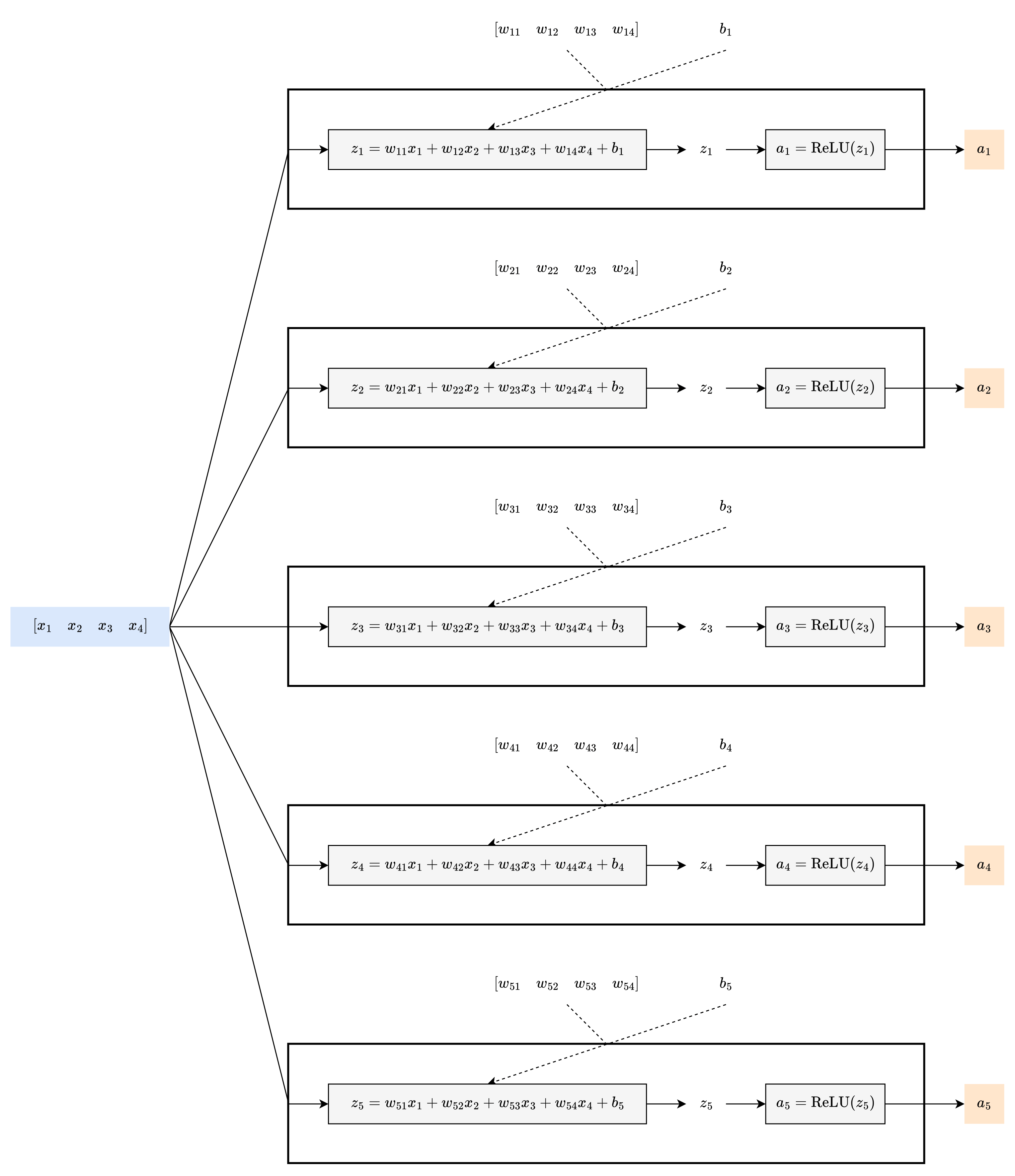
This layer has 4 inputs and 5 outputs.
Here, each neuron has different parameters—with different initial values:
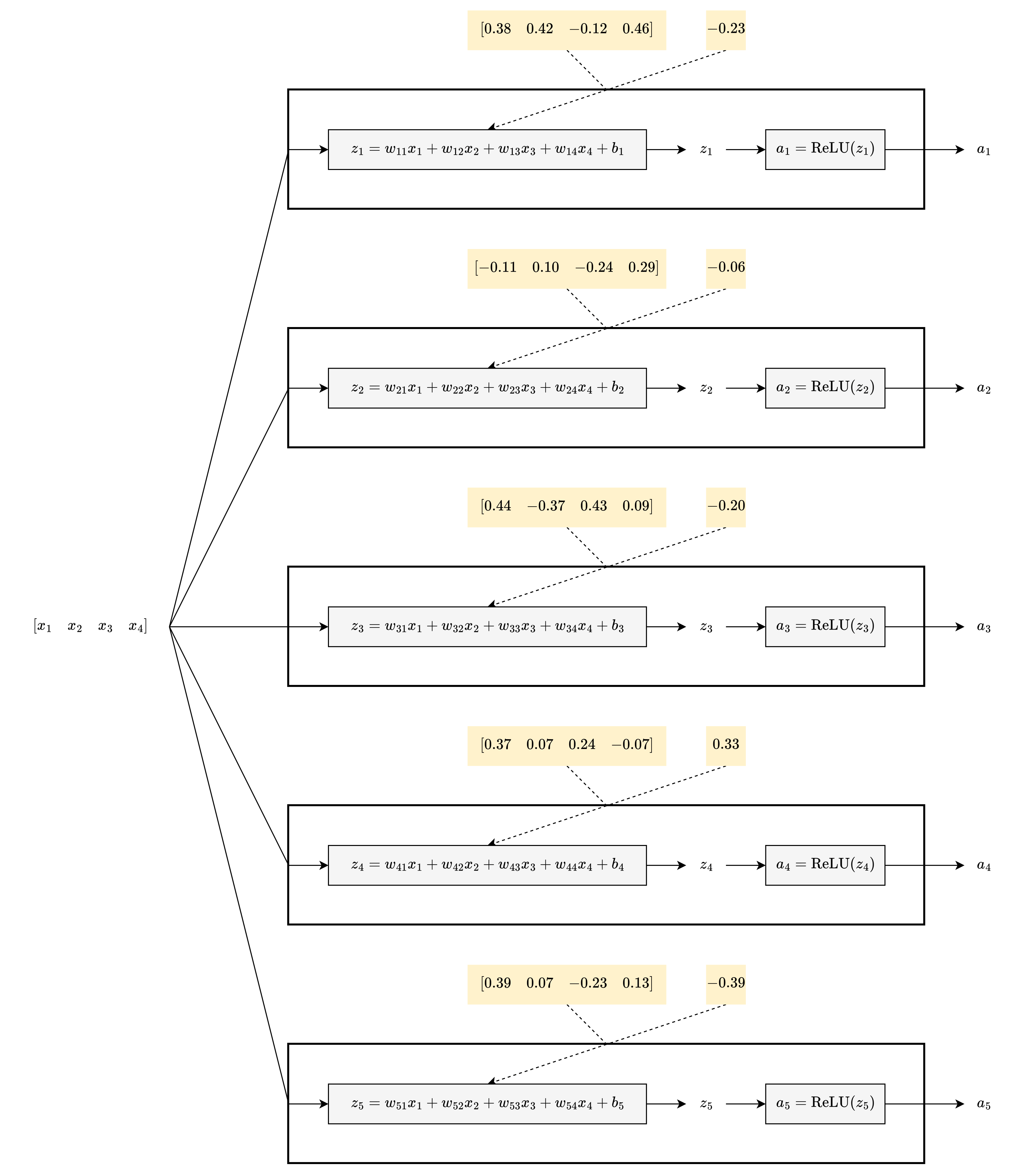
With different parameters for each neuron, when you feed the values from the input layer into the hidden layer…
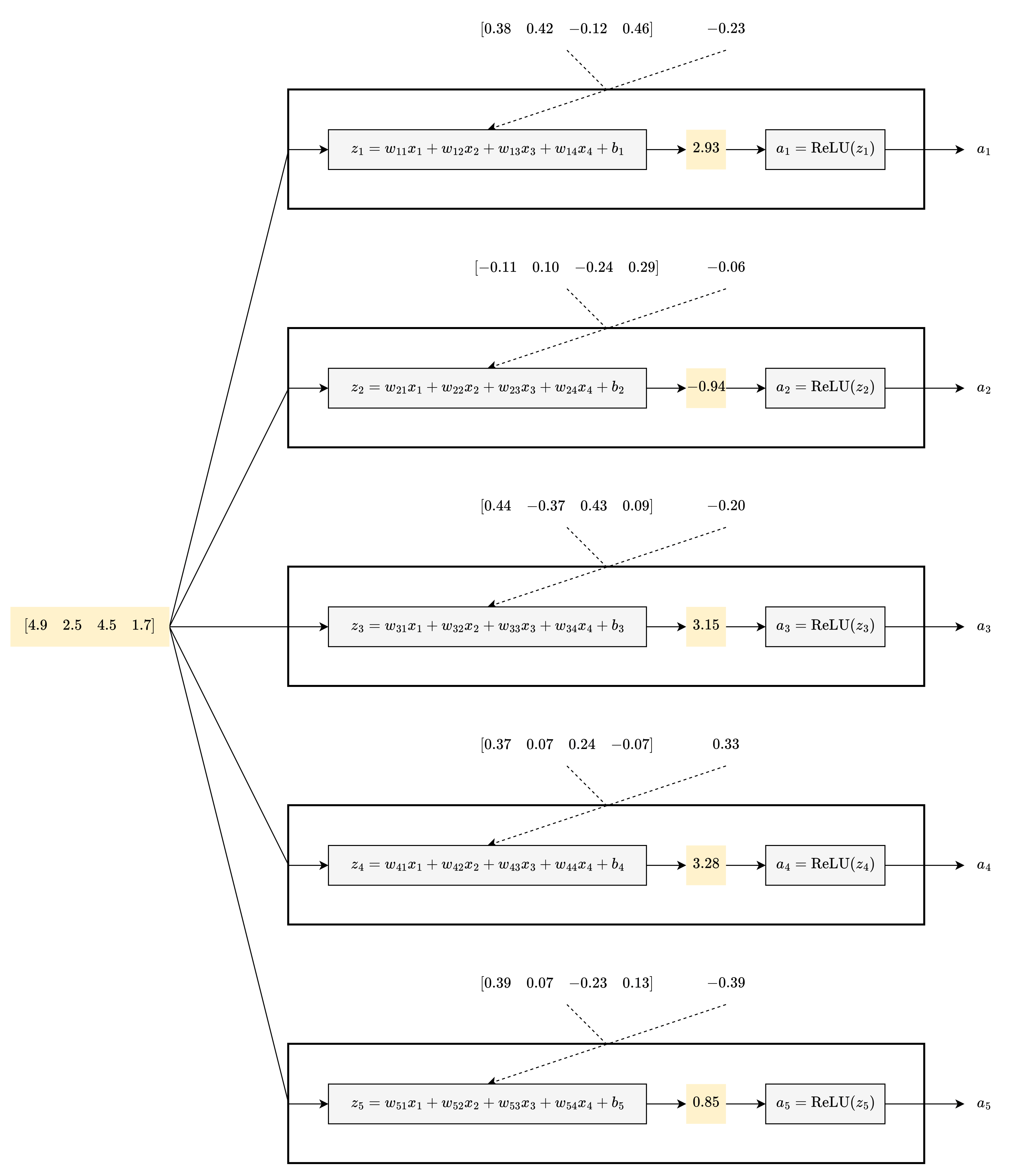
…each neuron combines those values in a different way.
When you continue through the second part of the hidden layer…
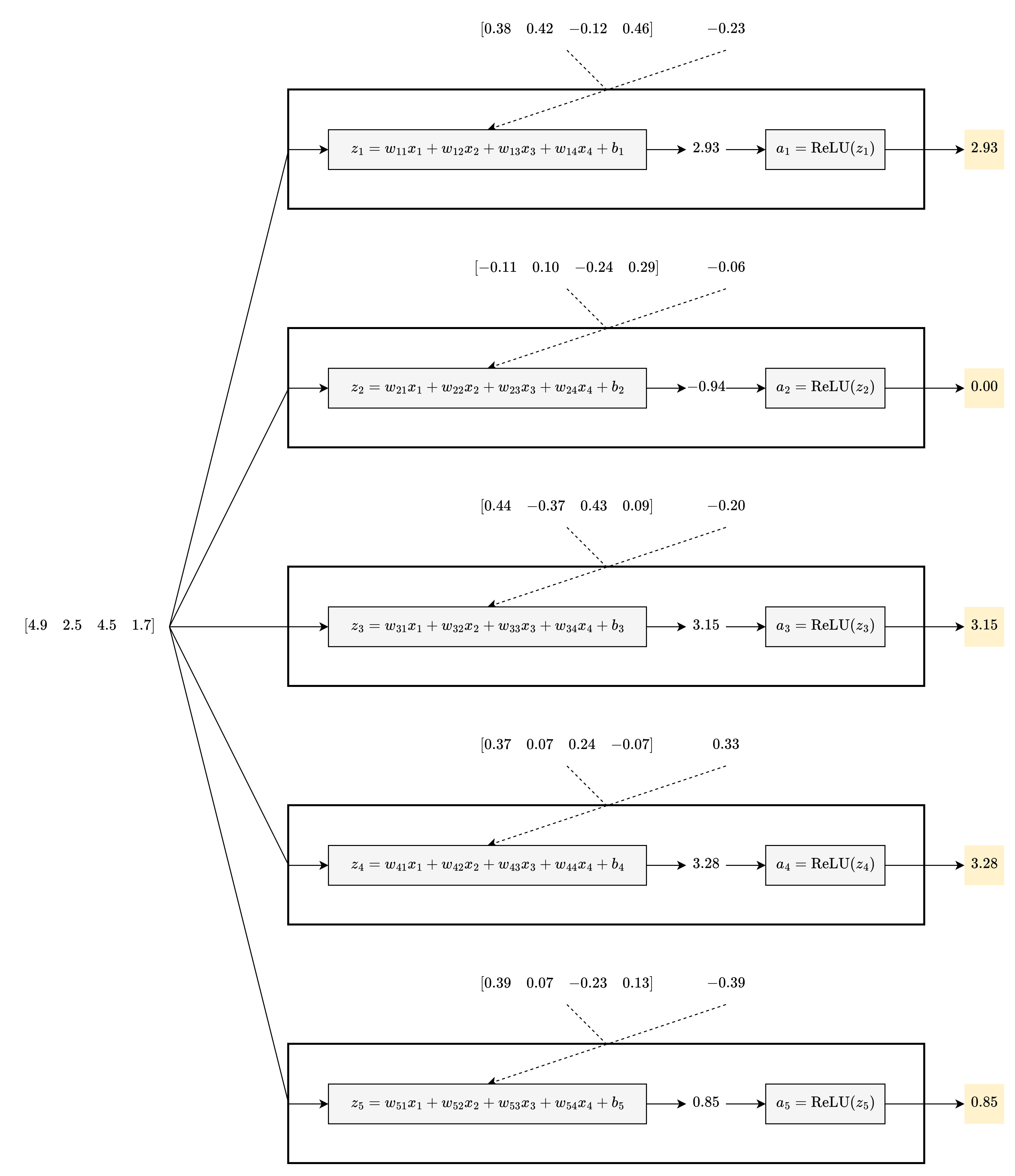
…4 neurons are activated, while 1 neuron (the second one) is not activated.
Model: Output Layer
The last stop is the output layer:
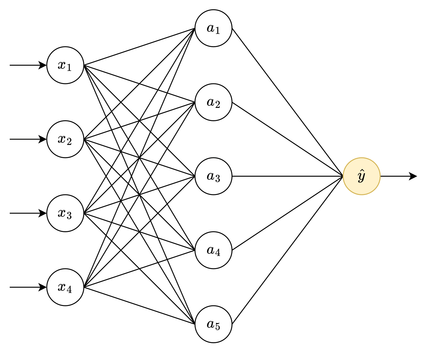
The output layer also has parameters, so how do you distinguish between the parameters for the hidden and output layers? Let’s look inside this layer:

Every parameter (and z) has a ⁽²⁾ next to it. (In a similar vein, you would also add ⁽¹⁾ to every parameter and the z’s in the hidden layer.)
As usual, the first step is to initialize the parameters:

When you feed the values from the hidden layer into the output layer…

…the first part feels familiar: it’s another linear combination.
For the second part, what is σ (sigmoid)? It’s easier to explain when you see it:

Sigmoid converts a number to a probability: 0 is 0%, and 1 is 100%. ŷ is a probability. In this case, that probability is approximately 22%:

There is also a term for the number that gets converted to a probability: z⁽²⁾ is a logit.
Decision Time
Finally, when this neural network needs to make a yes/no choice, it will choose “yes” when that probability is above 50%. In this case, with a probability of 22%, this neural network will choose “not iris virginica.” However, this sample actually is iris virginica.
4. Training the Artificial Brain
You know how this neural network works, but you do not know if it works. If you train this neural network, will it produce useful predictions or hallucinations?
Loss: One Sample
To train this neural network against your sample, you need to calculate loss for that sample. Here is the loss diagram for one sample:
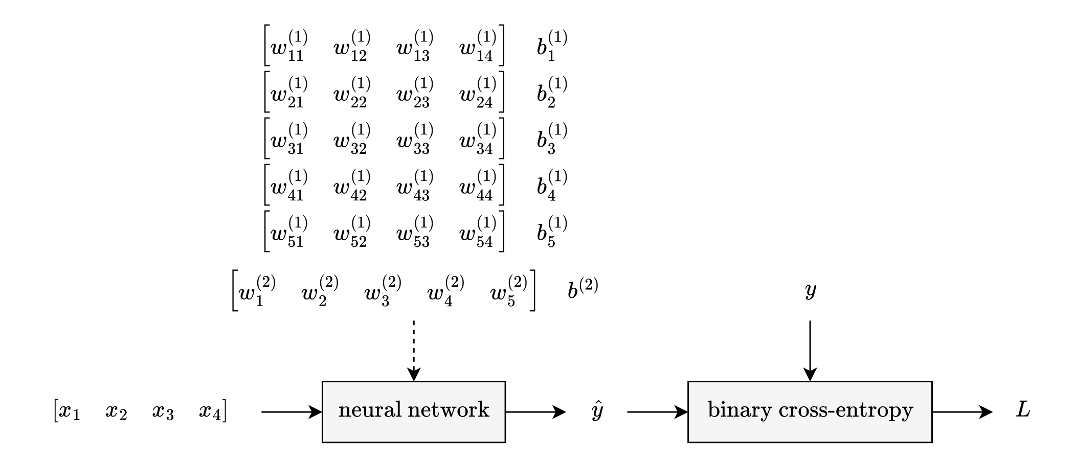
You may have noticed that the w⁽¹⁾’s form a rectangle, so let’s group them as such:
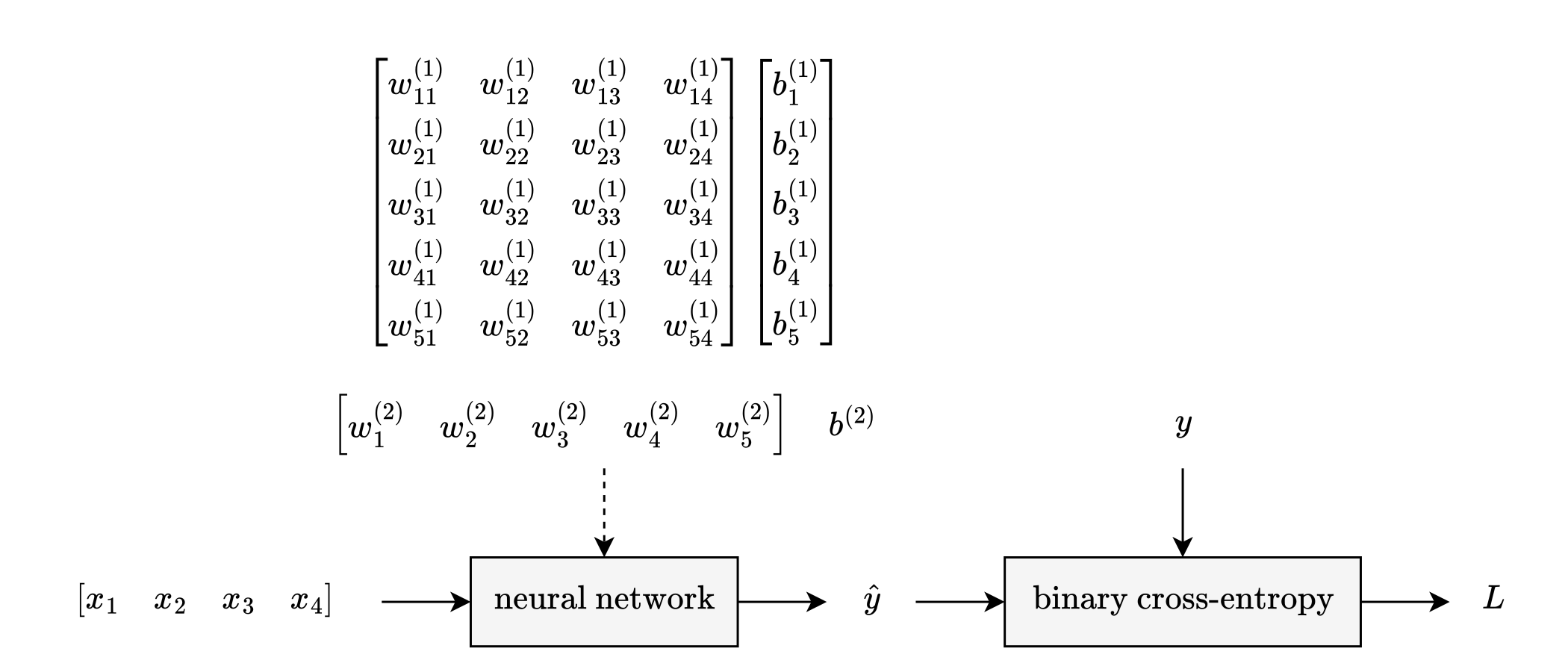
The fancy term for a rectangular collection of values is a matrix.
During part 3, you actually filled in most of this diagram:
First, you initialized the parameters to small random values:
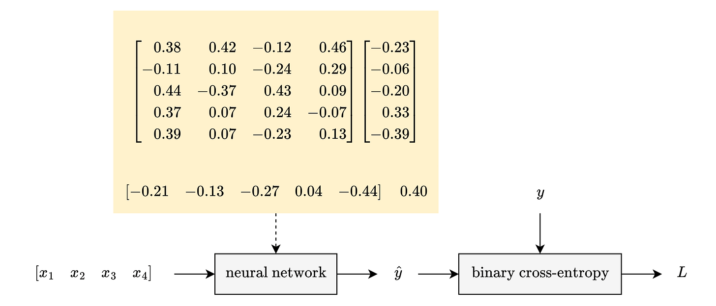
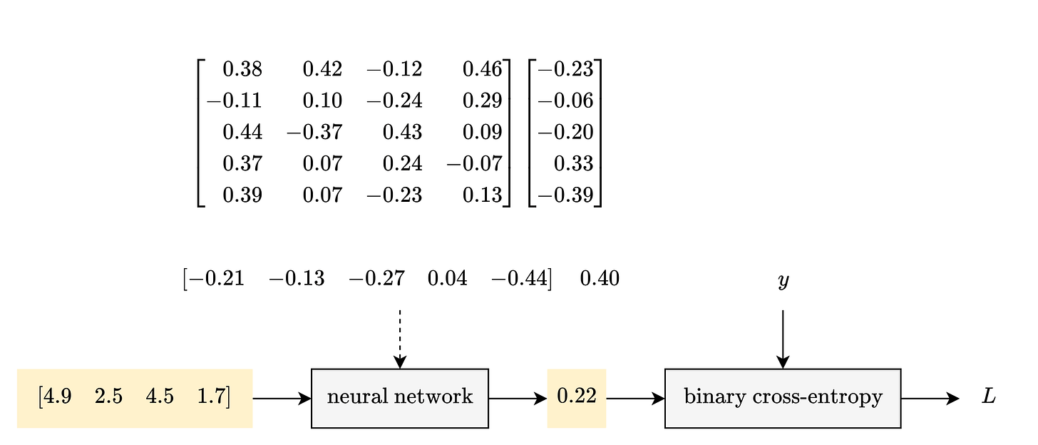
When you fed your sample into this neural network, it produced a prediction: a 22% chance that this sample is iris virginica:
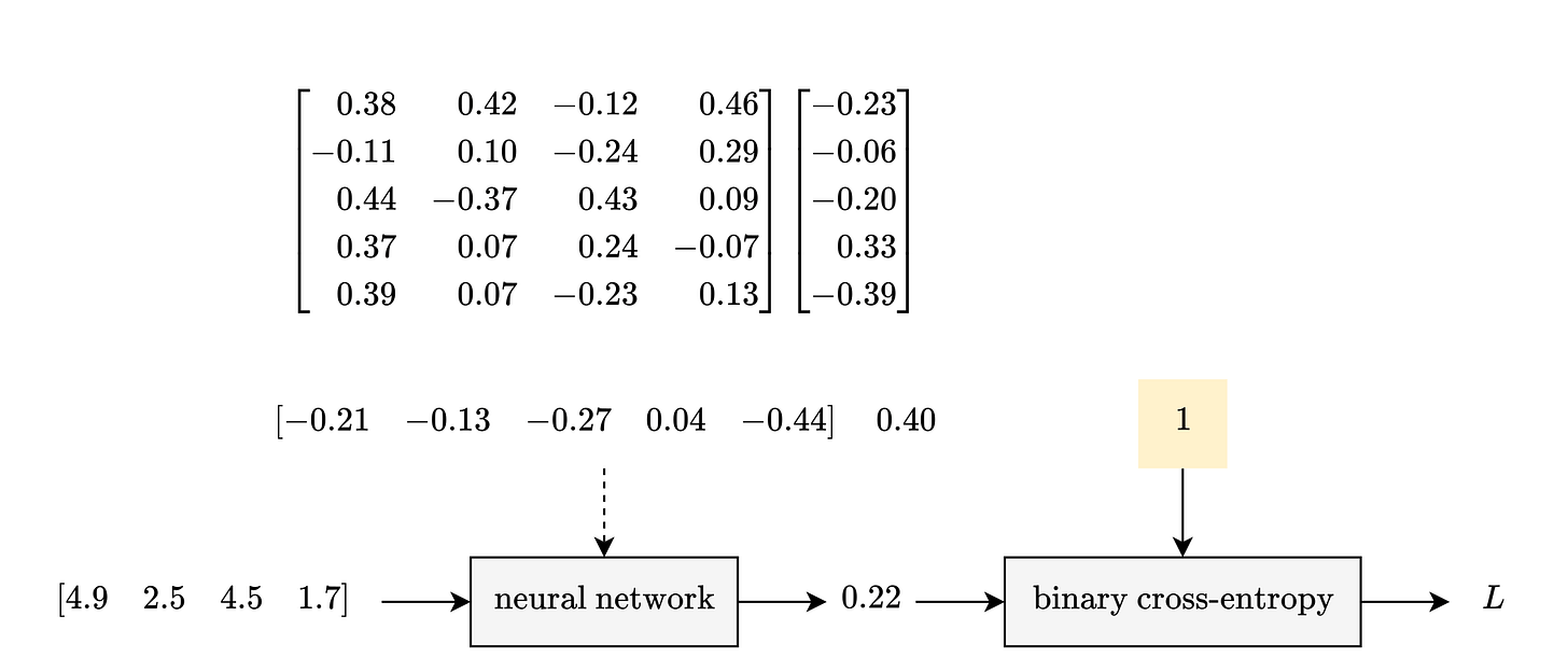
At the end, you learned that this sample is iris virginica. Therefore, the target is 1; there is a 100% chance that this sample is iris virginica:
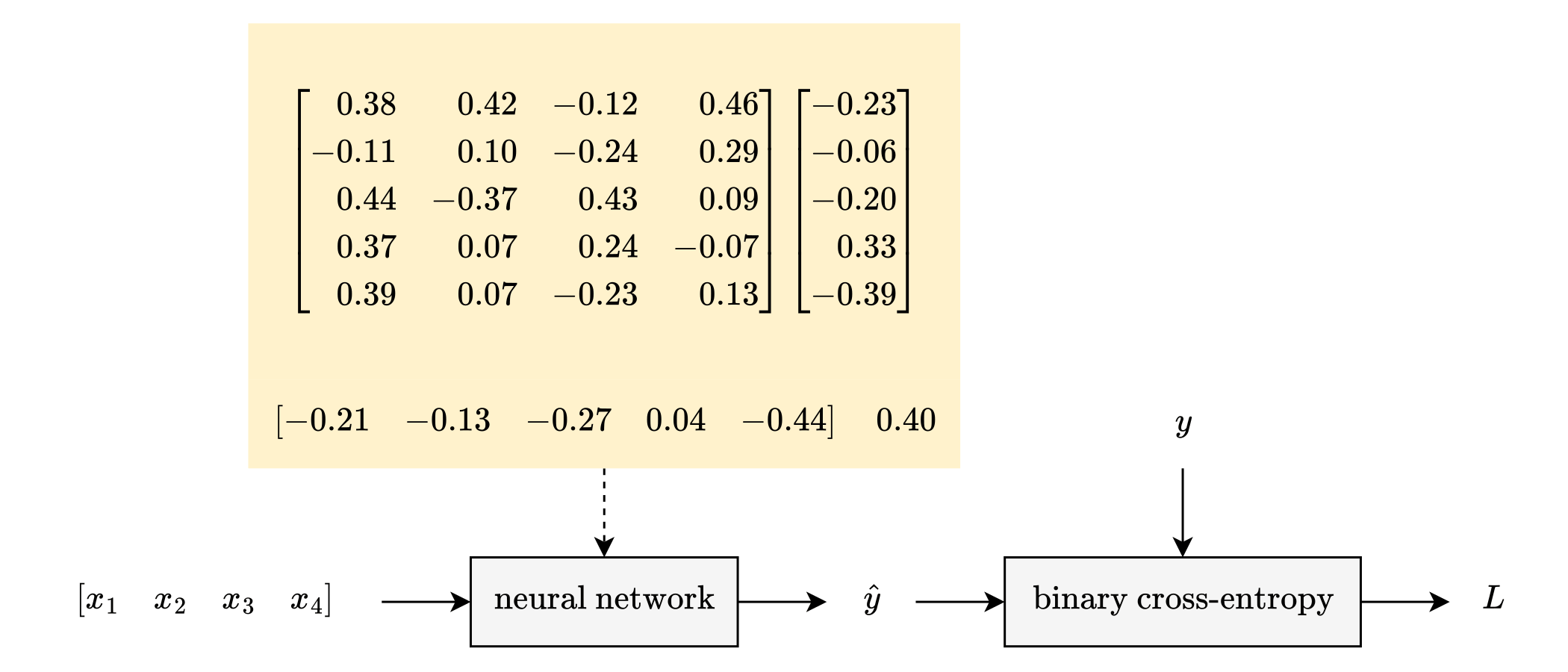
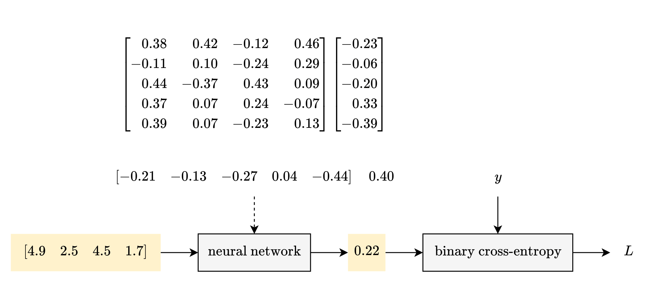
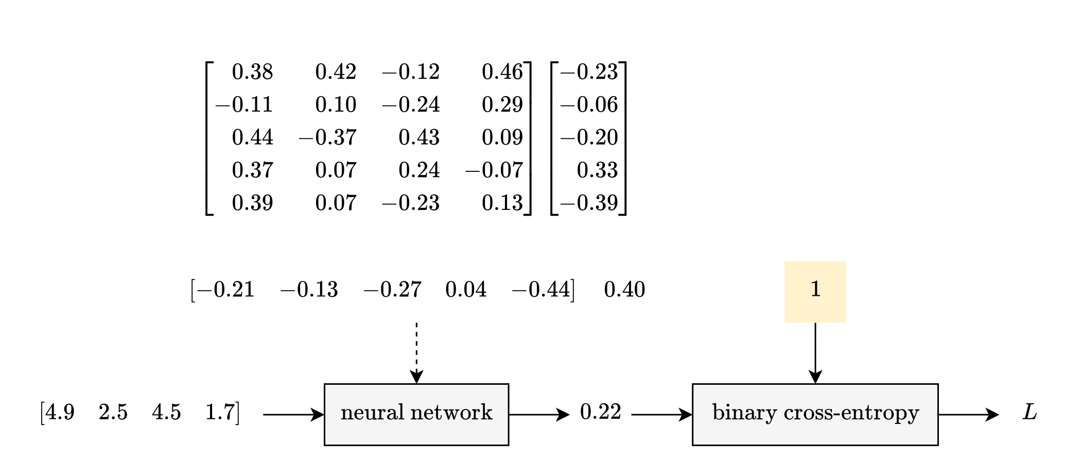
As for binary cross-entropy, it’s easier to explain when you see it:
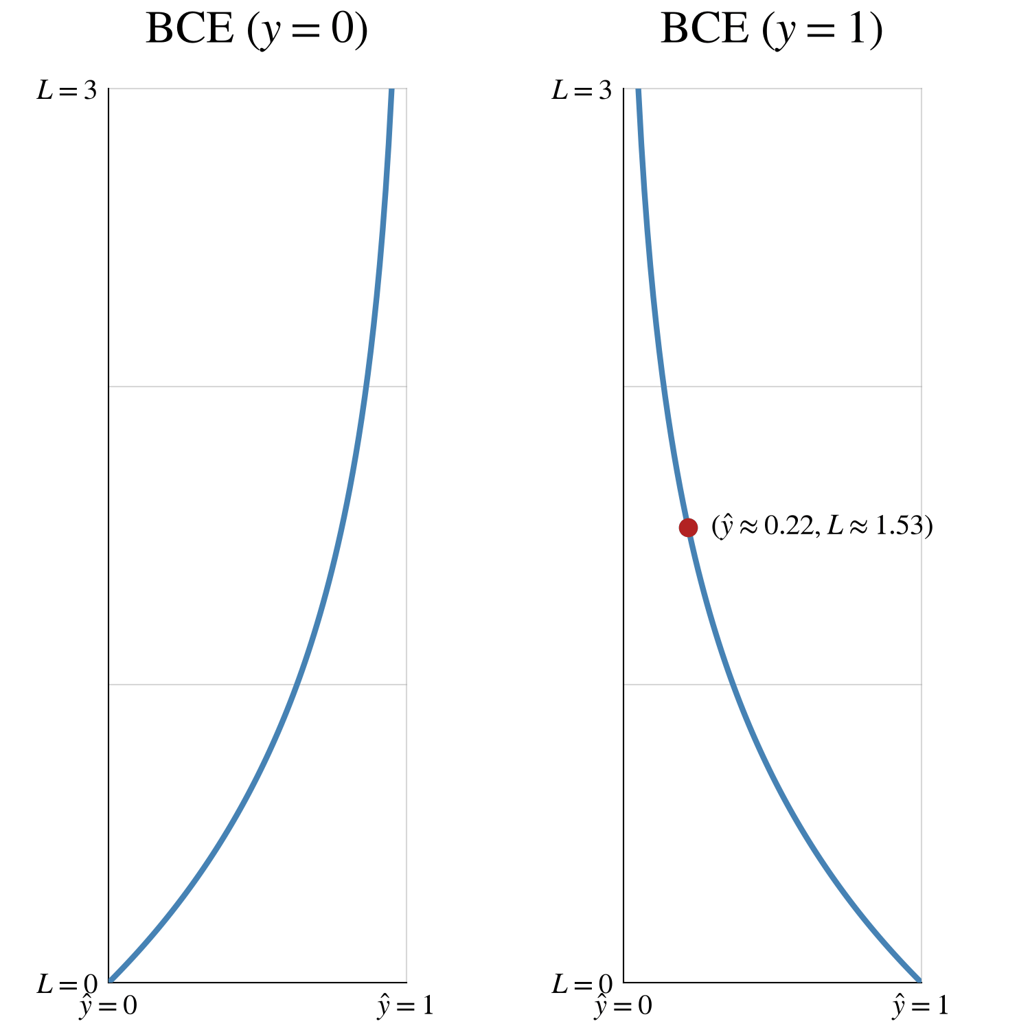
When the target is 0%, the loss is lower at 10% and higher at 90%.
When the target is 100%, the loss is lower at 90% and higher at 10%.
In this case, 22% is pretty far from 100%, so the loss is higher: approximately 1.53:
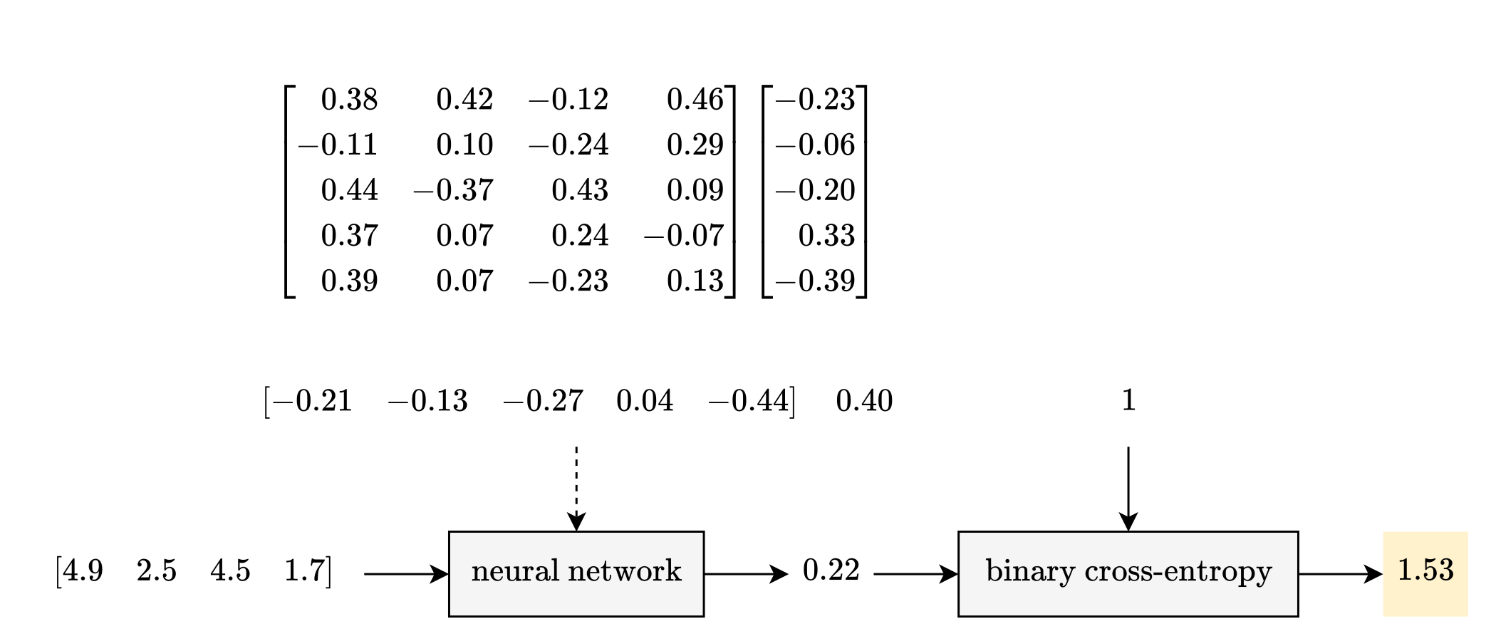
This process to calculate loss is often called the forward pass.
Loss: Training Data
Of course, you need more than one sample to train a model, so you will need to collect iris flowers and take their measurements. Just kidding. You can use the iris dataset:
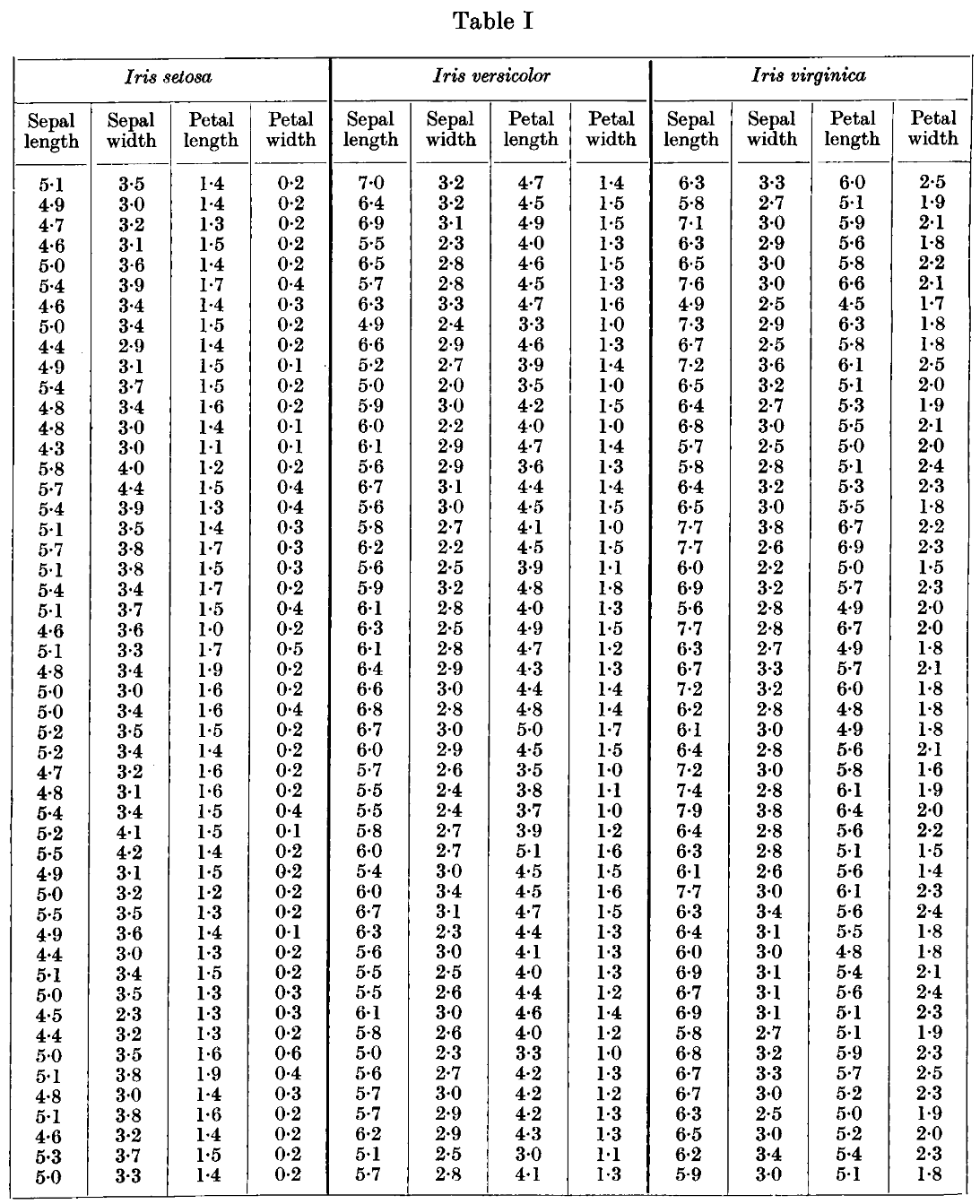
Thanks to this dataset, you have 120 samples to train your model. In fact, that sample you’ve been using comes from this dataset (7th row for the iris virginica column).
As a constructively lazy engineer, though, I am not creating a diagram with 480 x’s.
To create a loss diagram for multiple samples, you need to start representing matrices with a single letter. Let’s start with the loss diagram for one sample:

It’s the same diagram, but some of the notation has changed:
W⁽¹⁾ is a 5 × 4 matrix (5 rows, 4 columns), and b⁽¹⁾ is a 5 × 1 matrix.
w⁽²⁾ is a 1 × 5 matrix, and b⁽²⁾ is a single value.
x is a 1 × 4 matrix.
To support multiple samples, though, you do need to change the diagram:

X is now a 120 × 4 matrix.
ŷ and y are now both 120 × 1 matrices.
Is that legal? Can you feed a 120 × 4 matrix into this neural network? In short, yes.
For example, the hidden layer will do 600 linear combinations (120 samples × 5 neurons). With matrices, though, you can do 600 linear combinations with 1 equation:
You don’t need to know how this equation works; it involves matrix multiplication. But that is where GPUs get involved: GPUs can multiply matrices very quickly.
(To calculate binary cross-entropy for 120 samples, you would 1) calculate binary cross-entropy for each sample, and 2) combine 120 values into 1 value by taking the average.)
Finally, to ask a familiar question, what are the inputs in that loss diagram?

The inputs are the parameters.
The output is loss.
The features and targets are fixed by the training data.
This loss function has 31 inputs and 1 output.
Slope: Logit
With 31 inputs and 1 output, though, the loss function is a 32-dimensional hill. You cannot see a 32-dimensional hill; you are literally navigating this hill in the darkness.
And when the model is a neural network, I can no longer provide a simple equation to calculate the gradient.
If we look at just your sample, though, I can provide this equation:
To use this equation, recall the first step of gradient descent:
Calculate the loss at your current location (save all the values from this step):
If you saved those values from the forward pass, you can retrieve them here:
So what does this equation mean? Between the logit [z⁽²⁾] and loss [L], there were two steps: sigmoid and binary cross-entropy. You have seen both functions, but you have not seen what happens when you chain them together into a single function:
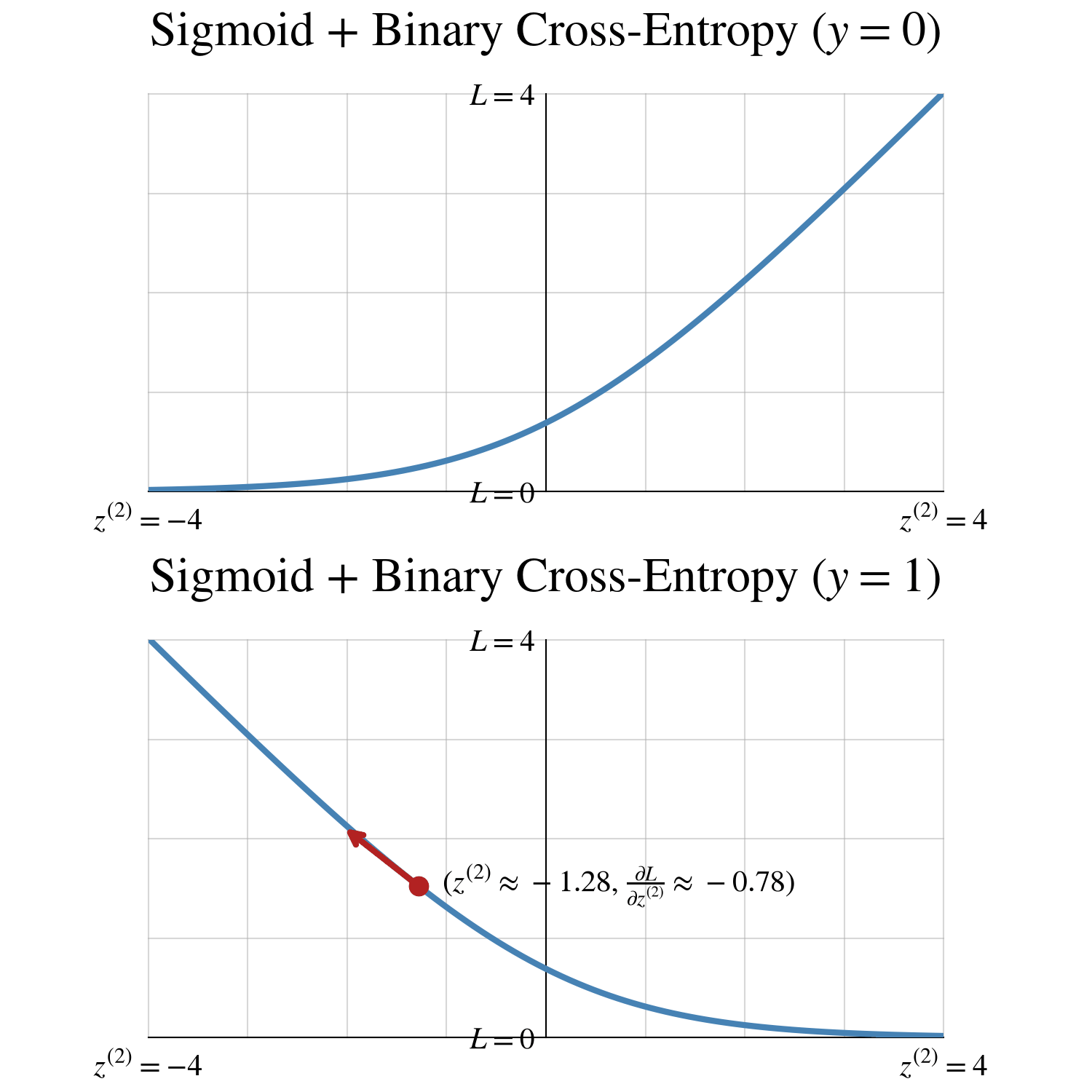
When the target is 0%, you travel downhill by decreasing the logit—which in turn decreases ŷ and brings it closer to 0%.
When the target is 100%, you travel downhill by increasing the logit—which in turn increases ŷ and brings it closer to 100%.
In this case, traveling downhill will increase the logit.
However, you cannot directly increase the logit; you can only directly change the parameters. To figure out which changes to the parameters will increase the logit, you must travel backward through the neural network by using backpropagation.
Slope: Output Layer
During the backward pass, the neural network is the same, but the goal has changed: calculating the gradient. Thus, the diagrams are the same, but for one change:

Each value has been replaced with a corresponding derivative. For example, a₁ has been replaced with ∂L/∂a₁. As you travel backward, you will eventually calculate the gradient: 31 derivatives for 31 parameters. (Those derivatives are shown in red text.)
You can start at the logit [z⁽²⁾], since you already calculated ∂L/∂z⁽²⁾:

From z⁽²⁾, though, how do you take a backward step to w⁽²⁾₁?
During the forward pass, the function in the gray box was a forward link to z⁽²⁾:
\(z^{(2)} = w^{(2)}_1 a_1 + w^{(2)}_2 a_2 + w^{(2)}_3 a_3 + w^{(2)}_4 a_4 + w^{(2)}_5 a_5 + b^{(2)}\)To create a backward link from z⁽²⁾ to w⁽²⁾₁, you convert that function to a corresponding derivative: ∂z⁽²⁾/∂w⁽²⁾₁. (I’ll calculate the derivative for you:)
\(\frac{\partial z^{(2)}}{\partial w^{(2)}_1} = a_1\)During the forward pass, a₁ was approximately 2.93:
\(\frac{\partial z^{(2)}}{\partial w^{(2)}_1} = a_1 \approx 2.93\)To use that backward link, though, you need another tool from calculus: the chain rule. (I’ll apply the chain rule for you:)
\(\frac{\partial L}{\partial w^{(2)}_1} = \frac{\partial L}{\partial z^{(2)}} \frac{\partial z^{(2)}}{\partial w^{(2)}_1}\)Here, you already calculated both derivatives on the right-hand side:
\(\frac{\partial L}{\partial w^{(2)}_1} = \frac{\partial L}{\partial z^{(2)}} \frac{\partial z^{(2)}}{\partial w^{(2)}_1} \approx -0.78 \cdot 2.93 \approx -2.30\)

In a similar vein, from z⁽²⁾, you can take 5 more steps to the other 5 parameters:

The remaining 25 parameters lie within the hidden layer. To reach the hidden layer, though, you must first reach the beginning of the output layer.
From z⁽²⁾, you can also take a step to a₁. Let’s walk through this step:
To create a backward link, convert the function to a derivative:
Function:
\(z^{(2)} = w^{(2)}_1 a_1 + w^{(2)}_2 a_2 + w^{(2)}_3 a_3 + w^{(2)}_4 a_4 + w^{(2)}_5 a_5 + b^{(2)}\)Derivative:
\(\frac{\partial z^{(2)}}{\partial a_1} = w^{(2)}_1\)During the forward pass, w⁽²⁾₁ was approximately -0.21:
\(\frac{\partial z^{(2)}}{\partial a_1} = w^{(2)}_1 \approx -0.21\)
To use that backward link, use the chain rule:
\(\frac{\partial L}{\partial a_1} = \frac{\partial L}{\partial z^{(2)}} \frac{\partial z^{(2)}}{\partial a_1} \approx -0.78 \cdot -0.21 \approx 0.16\)

In a similar vein, from z⁽²⁾, you can take 4 more steps to the other 4 a’s:

Slope: Hidden Layer
When you reach the beginning of the output layer, you also reach the end of the hidden layer—including the end of the neuron for a₁:

From a₁, you can take a step to z⁽¹⁾₁. Let’s walk through this step:
To create a backward link, convert the function to a derivative:
Function:
\(a_1 = \operatorname{ReLU}(z^{(1)}_1)\)Derivative:
\(\frac{\partial a_1}{\partial z^{(1)}_1} = \begin{cases} 1, & \text{if } z^{(1)}_1 > 0 \\ 0, & \text{if } z^{(1)}_1 \le 0 \end{cases}\)During the forward pass, z⁽¹⁾₁ was approximately 2.93:
\(\frac{\partial a_1}{\partial z^{(1)}_1} = \begin{cases} 1, & \text{if } z^{(1)}_1 > 0 \\ 0, & \text{if } z^{(1)}_1 \le 0 \end{cases} = \begin{cases} 1, & \text{if } 2.93 > 0 \\ 0, & \text{if } 2.93 \le 0 \end{cases} = 1\)
To use that backward link, use the chain rule:
\(\frac{\partial L}{\partial z^{(1)}_1} = \frac{\partial L}{\partial a_1} \frac{\partial a_1}{\partial z^{(1)}_1} \approx 0.16 \cdot 1 \approx 0.16\)

From z⁽¹⁾₁, you can take 5 steps to the 5 parameters:

To reach the other 20 parameters, you can repeat those 6 steps for the other 4 neurons:
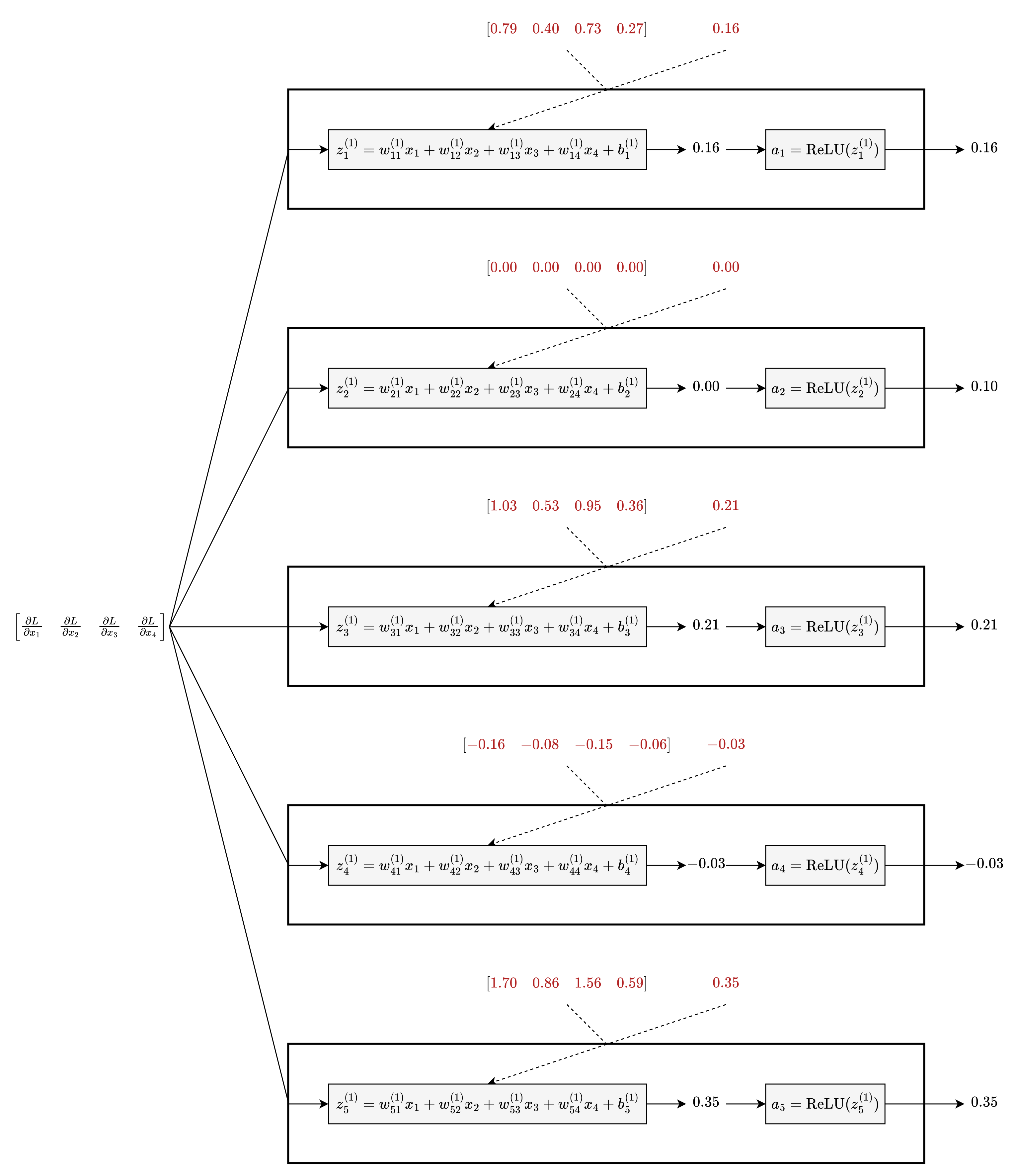
You have now calculated the derivatives for all 31 parameters…at least for 1 sample.
Slope: Training Data
When you train this neural network, you will backpropagate 120 samples in a single pass. It’s a similar process, but it involves matrix calculus.
The end result, however, is effectively the same as 1) calculating 120 gradients for 120 samples, and 2) combining those 120 gradients into an average gradient.
Backpropagation is also where the analogy to the human brain ends; the human brain does not learn via backpropagation. The learning process is an artificial process.
Learn
While you cannot see a 32-dimensional hill, you can see the changes to the parameters:
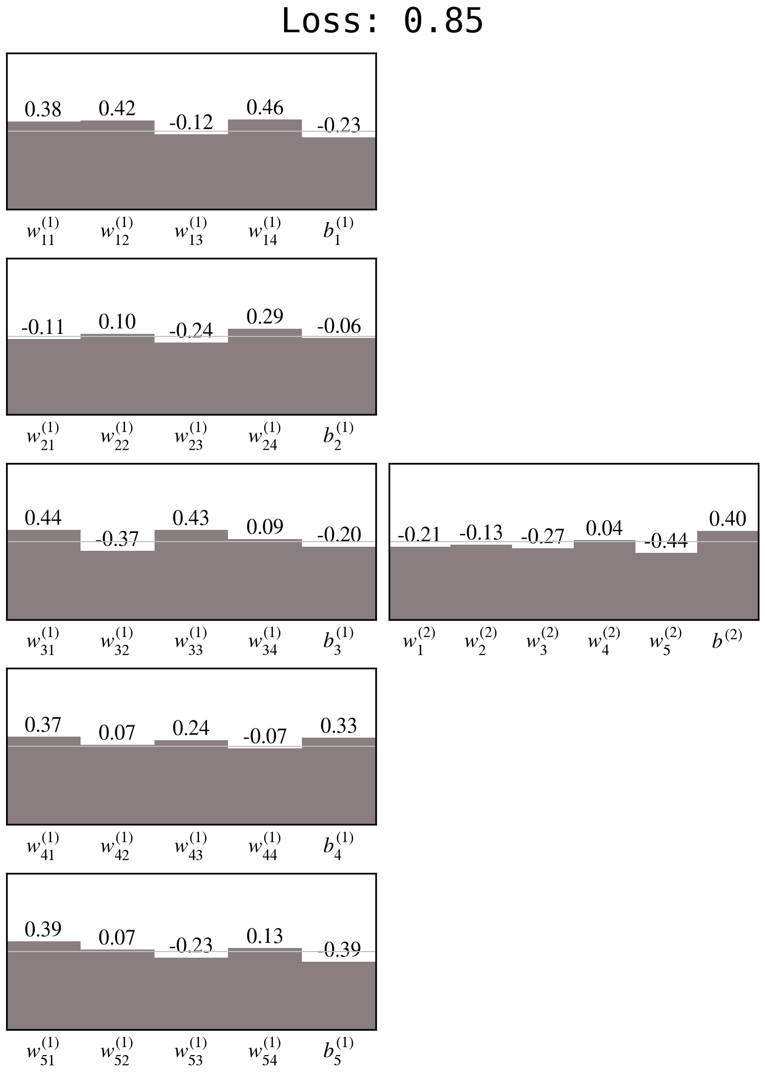
This video shows what happens when you train this neural network for 3000 steps:
After 3000 steps, here are the trained parameters:
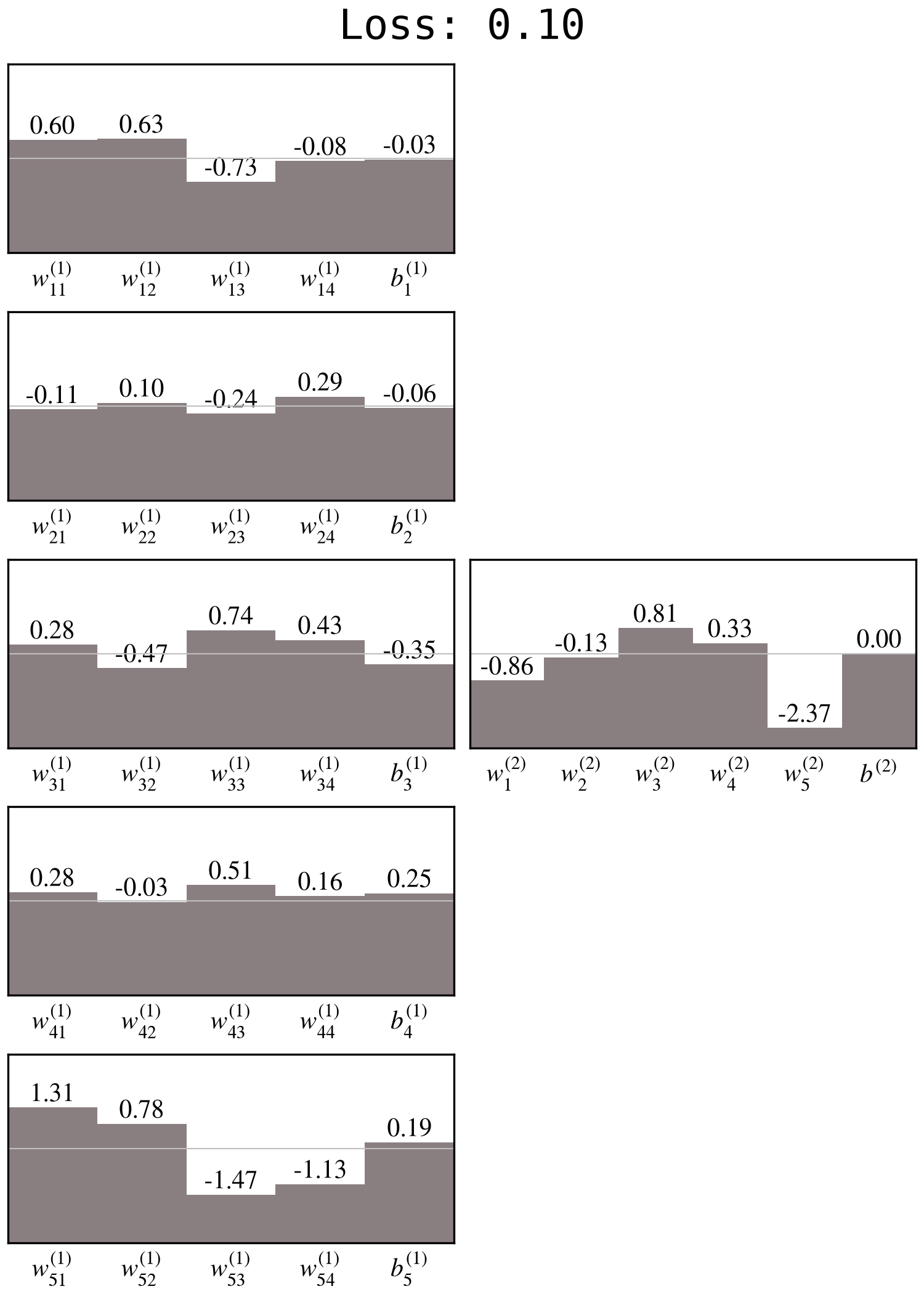
With trained parameters, the neural network’s prediction for your sample changes from 22% to 97%; it correctly chooses “iris virginica.” As for the training data, it makes the correct choice for 117/120 samples: 97.5% accuracy.
Test
So will this neural network work in real life? In real life, it will see iris flowers that are not in the training data. And I just so happen to have 30 such flowers.
The iris dataset actually has 150 samples. However, I held back 30 samples, and only gave you 120 samples to train the neural network. This is called a train-test split.
If you feed those 30 test samples into the neural network, it makes the correct choice for 100% of those flowers. It’s a real result that was produced by an artificial process.
Epilogue: Advanced Thing-Labeling
The iris example had 31 parameters, but real-life neural networks can have millions, billions, or even trillions of parameters. But while a lot does change with these giant neural networks, three things remain the same:
AI is a giant math equation.
The training data catechizes the bot.
The learning process is an artificial process.
Real-life neural networks have multiple hidden layers, and they also have different types of hidden layers: image processing may use convolutional layers, while chatbots may use transformers. But if you knew how convolutional layers and transformers work, you would also know that they’re still math equations.
As for large language models [LLMs] like ChatGPT, they are also thing-labelers: the thing is the previous words in the conversation, and the label is the next word. (I’m omitting some technical details like tokenization, but that’s the basic idea.)
LLMs go through multiple phases of training: each phase has a different way of calculating loss, and each phase has its own training data. But while an LLM’s behavior is not 100% predictable—minimizing loss can produce some unexpected results—that behavior is still downstream of the training data.
(If you want to know more about how chatbots work, Eric Silberstein has written a great e-book there—though it is targeted at more of a STEM audience.)
And neural networks, including LLMs, “learn” through the following process:
a forward pass to calculate loss
a backward pass to calculate the gradient
an update to the parameters using gradient descent (or Adam or Muon)
With the right architecture and the right parameters, neural networks can produce some magical results, but these results were made with math, not magic.
Appendix: Multiple-Choice Questions
When the label consists of more than two choices, the task is a multiclass classification task. And the iris example was originally a multiclass classification task; the label was either iris setosa, iris versicolor, or iris virginica.
(LLMs are also an example of multiclass classification.)
Model: Neural Network
Here is the neural network for the multiclass model:
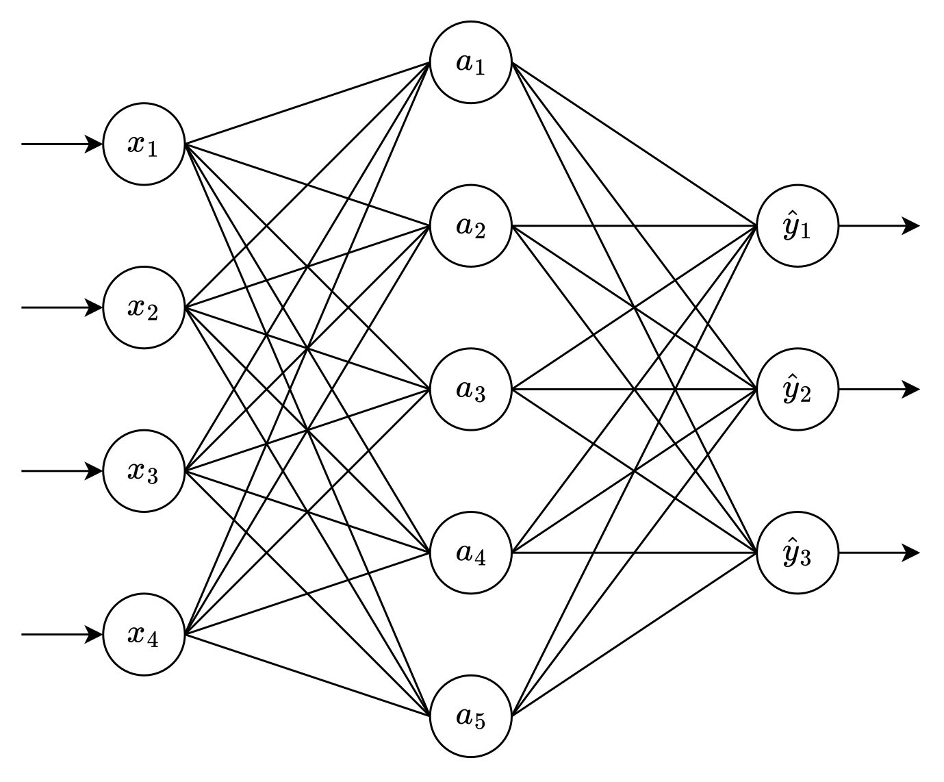
The output layer now has three neurons: one for each choice (or class):
ŷ₁: iris setosa
ŷ₂: iris versicolor
ŷ₃: iris virginica
Model: Output Layer
When you feed your sample into this neural network, everything remains the same through the input and hidden layers. The changes occur in the output layer:
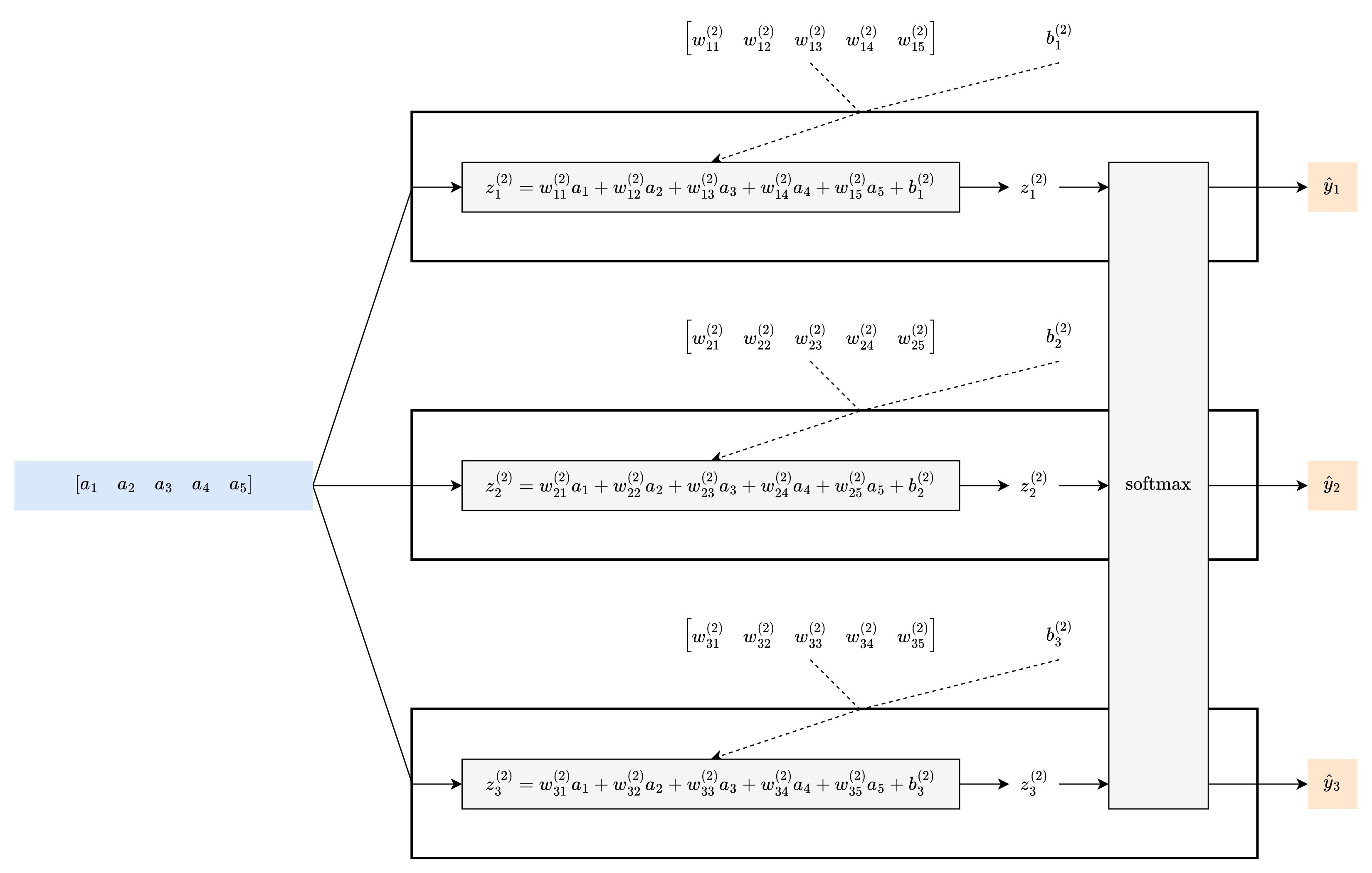
As usual, you first initialize the parameters; each neuron has its own parameters:
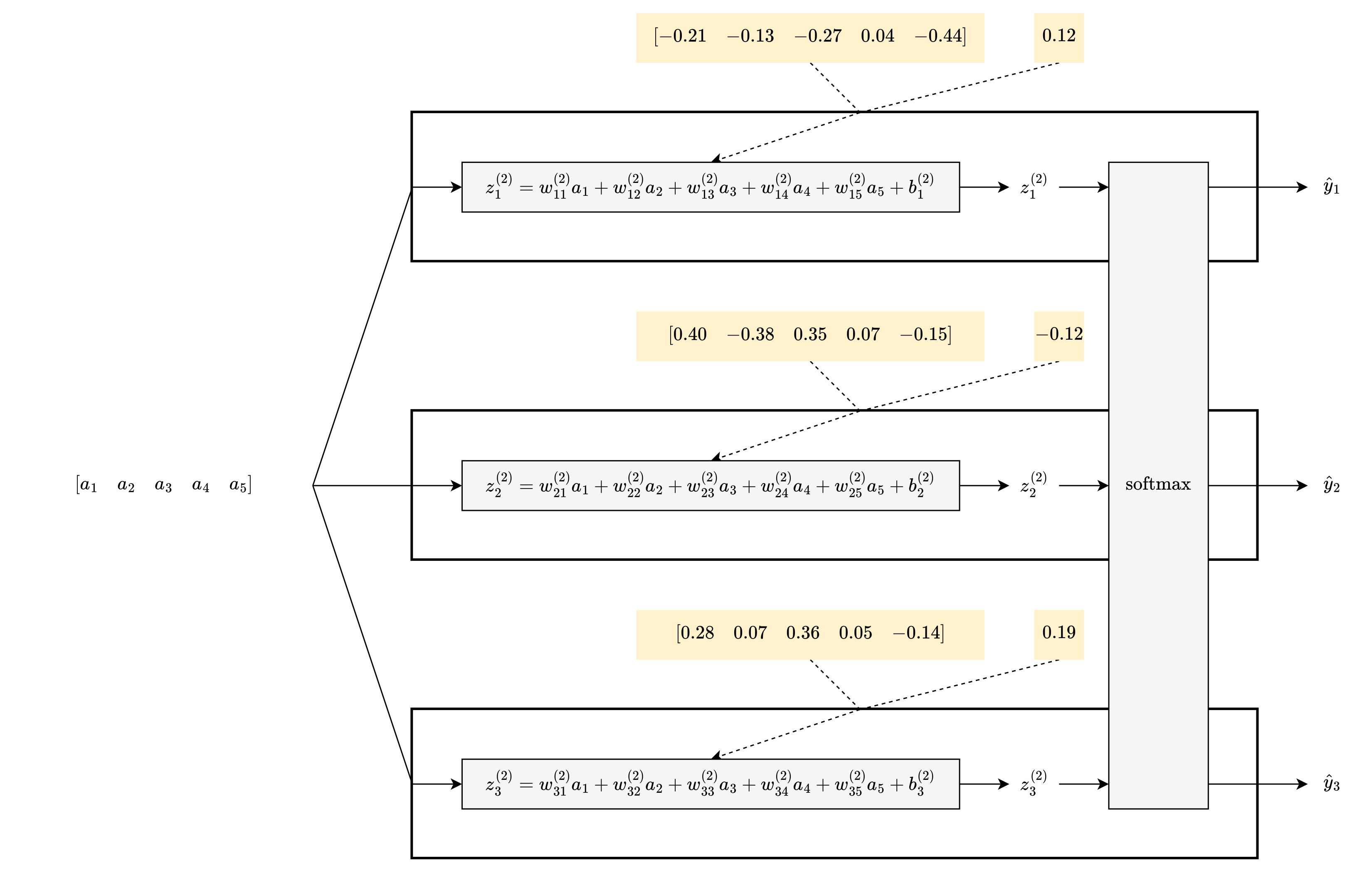
When you feed the values from the hidden layer into the output layer, the first part is still a linear combination for each neuron:
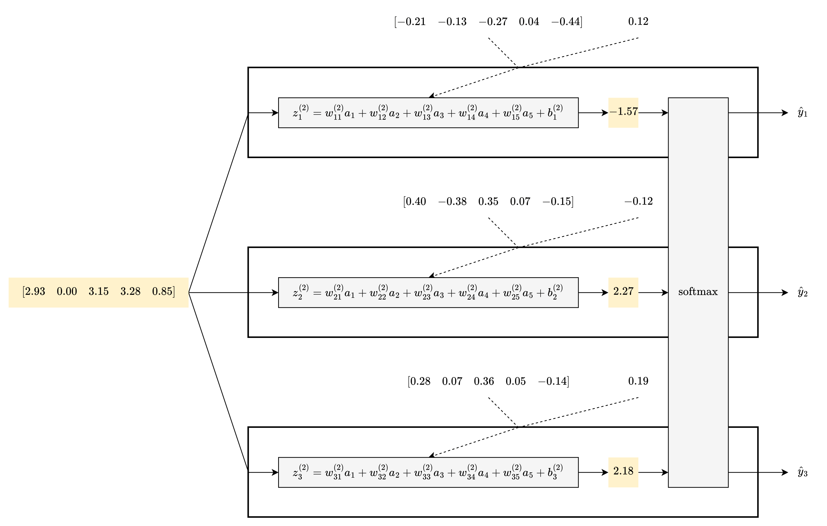
As for the second part, what is softmax? Softmax has 3 inputs and 3 outputs; you can’t see it since it’s a 6D function. But if you see the outputs, you can figure it out:
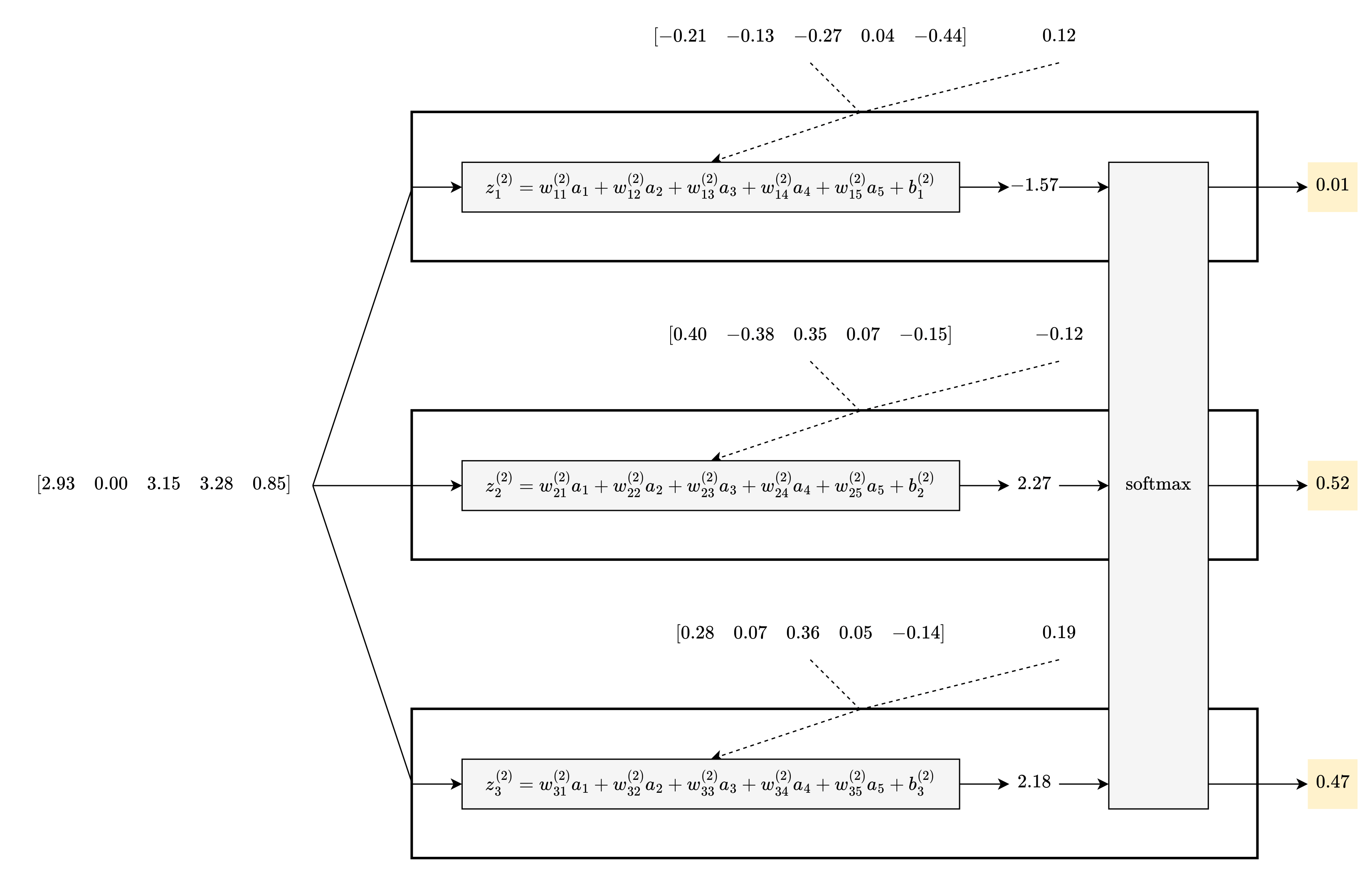
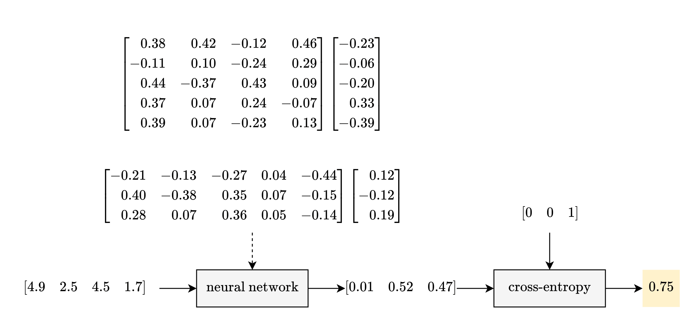
Softmax converts 3 logits to 3 probabilities. In this case, there is a 1% chance for iris setosa, a 52% chance for iris versicolor, and a 47% chance for iris virginica.
Finally, when this neural network needs to make a choice, it will choose the class with the highest probability. In this case, it will choose iris versicolor.
Loss: One Sample
Here is the loss diagram for one sample:
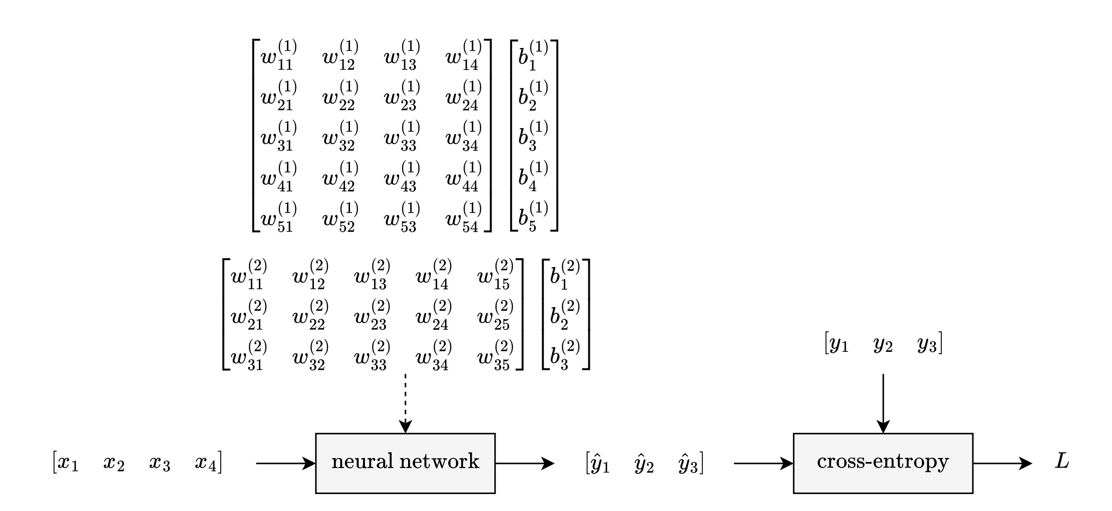
As usual, you first initialize the parameters:
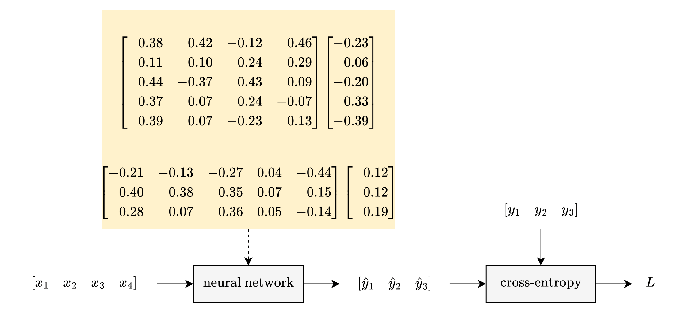
When you feed your sample into this model, the prediction is now a 1 × 3 matrix:
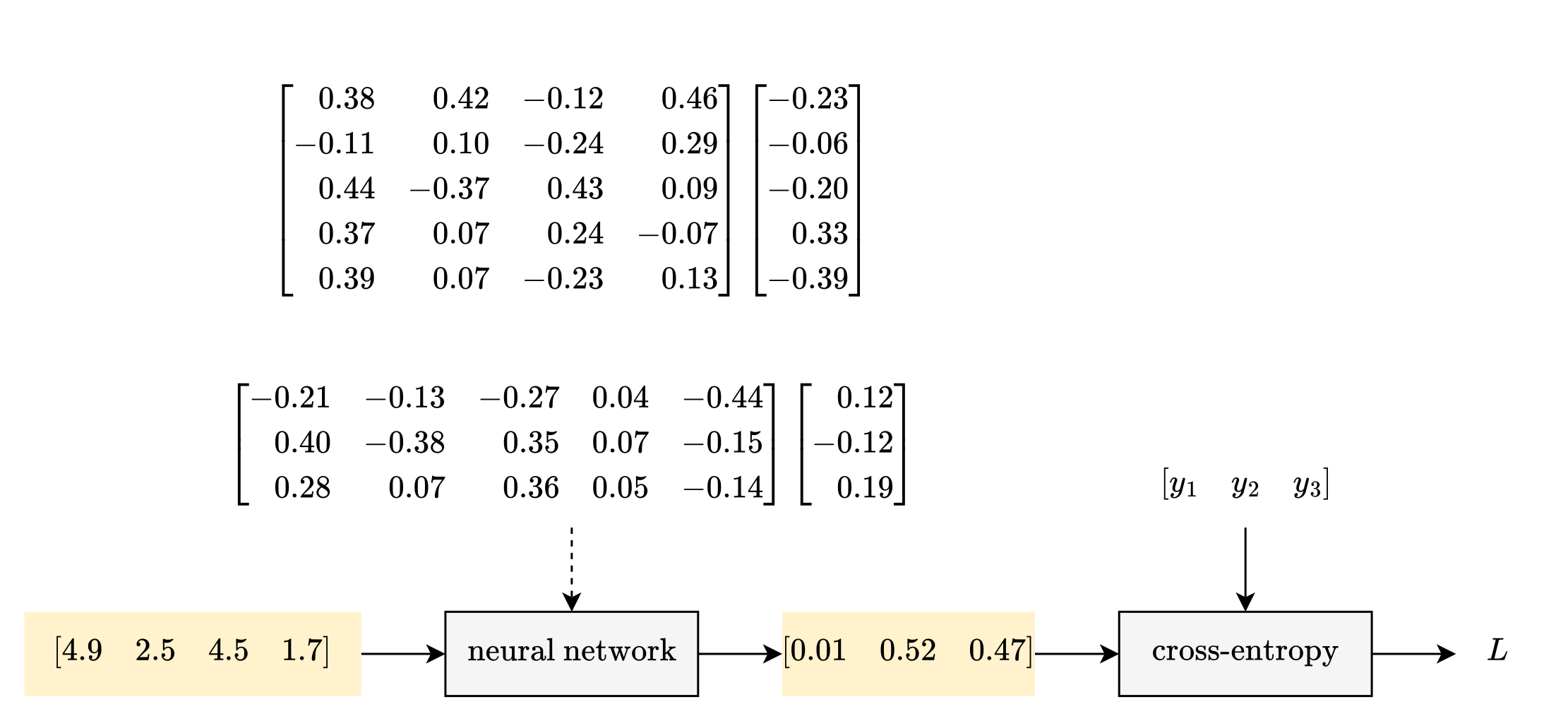
The target is also a 1 × 3 matrix. Since your sample is iris virginica, the target is a 100% chance for iris virginica [y₃] and a 0% chance for the other two classes:
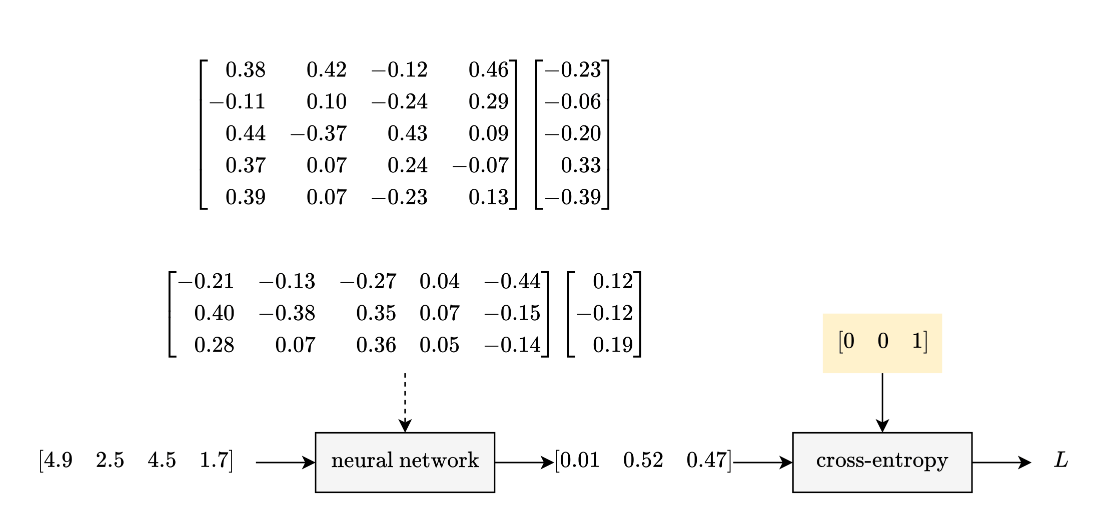
As for cross-entropy, it only compares the prediction and target for the correct class. In this case, cross-entropy compares ŷ₃ to y₃. This comparison will look familiar:
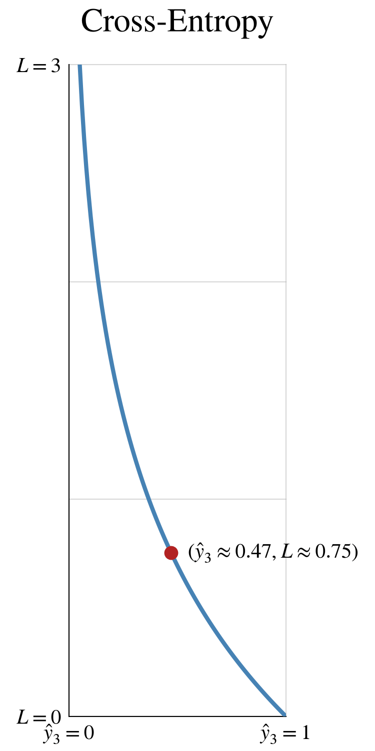
It is the same shape as binary cross-entropy when the target is 100%. In this case, 47% is fairly far from 100%, so the loss is approximately 0.75:
Loss: Training Data
Here is the loss diagram for multiple samples:

If you have m samples (in this case, m is 120), here are the shapes of the matrices:
W⁽¹⁾ is a 5 × 4 matrix, and b⁽¹⁾ is a 5 × 1 matrix.
W⁽²⁾ is a 3 × 5 matrix, and b⁽²⁾ is a 3 × 1 matrix.
X is an m × 4 matrix.
Ŷ and Y are both m × 3 matrices.
L is a single value.
Slope: Logits
If you chain softmax and cross-entropy together, the result is a function with 3 inputs and 1 output. You cannot see a 4D function, but this equation will look familiar:
(This is actually a 1 × 3 matrix, but the equation is more readable with a 3 × 1 matrix.)
With 3 logits, there are two ways to travel downhill:
increase the logit for iris virginica [z⁽²⁾₃]
decrease the logit for iris setosa [z⁽²⁾₁] or iris versicolor [z⁽²⁾₂]
With softmax, both changes would increase ŷ₃ and bring it closer to 100%.
Slope: Output Layer
Let’s backpropagate your sample through the output layer:
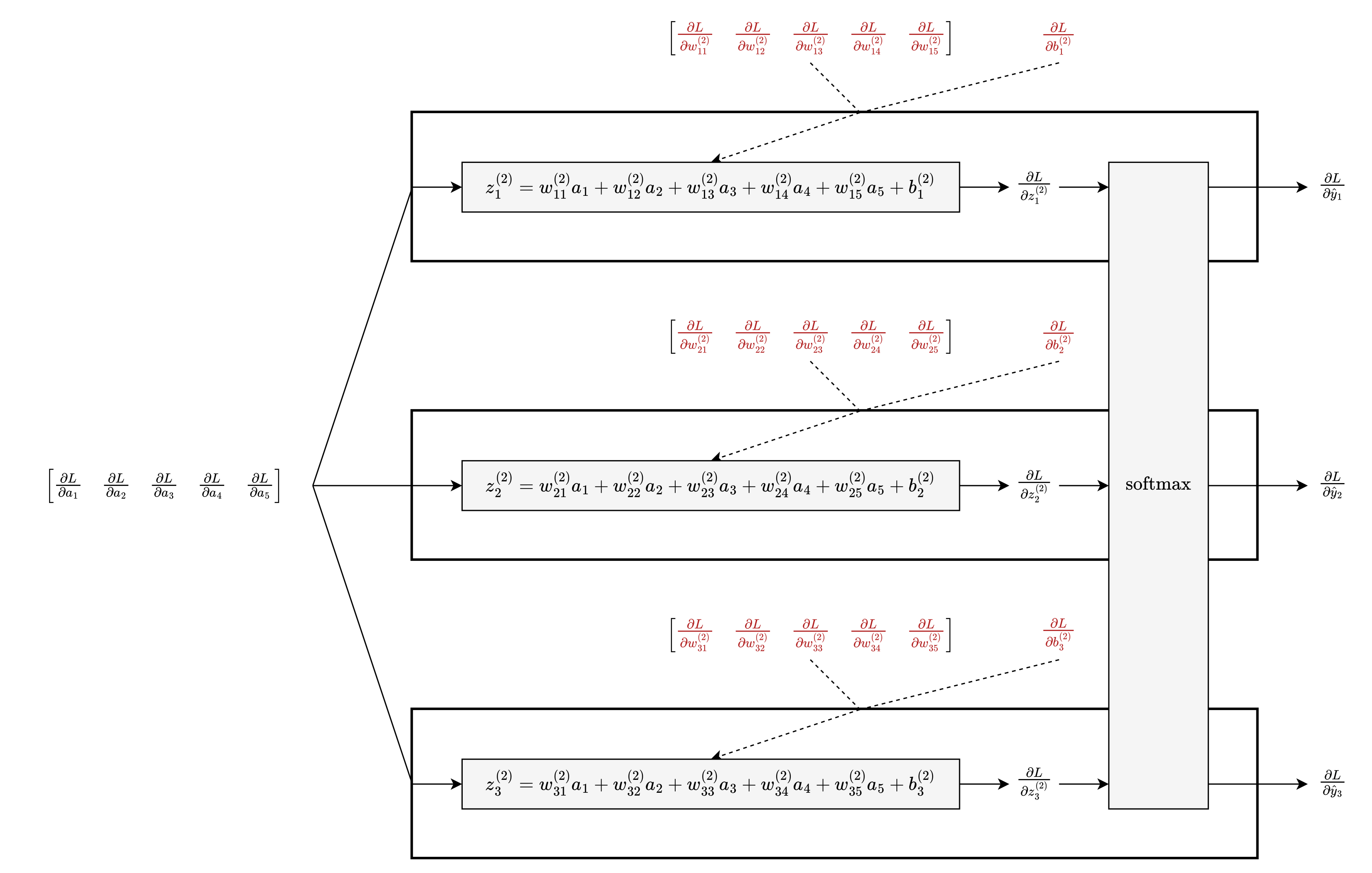
As before, you start with the logits:
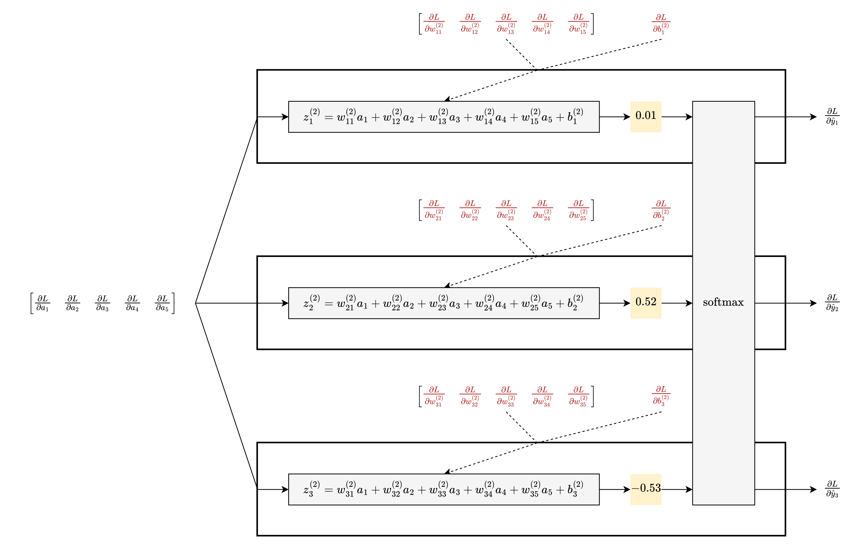
As before, from each logit, you can take 6 steps to the 6 parameters of that neuron:
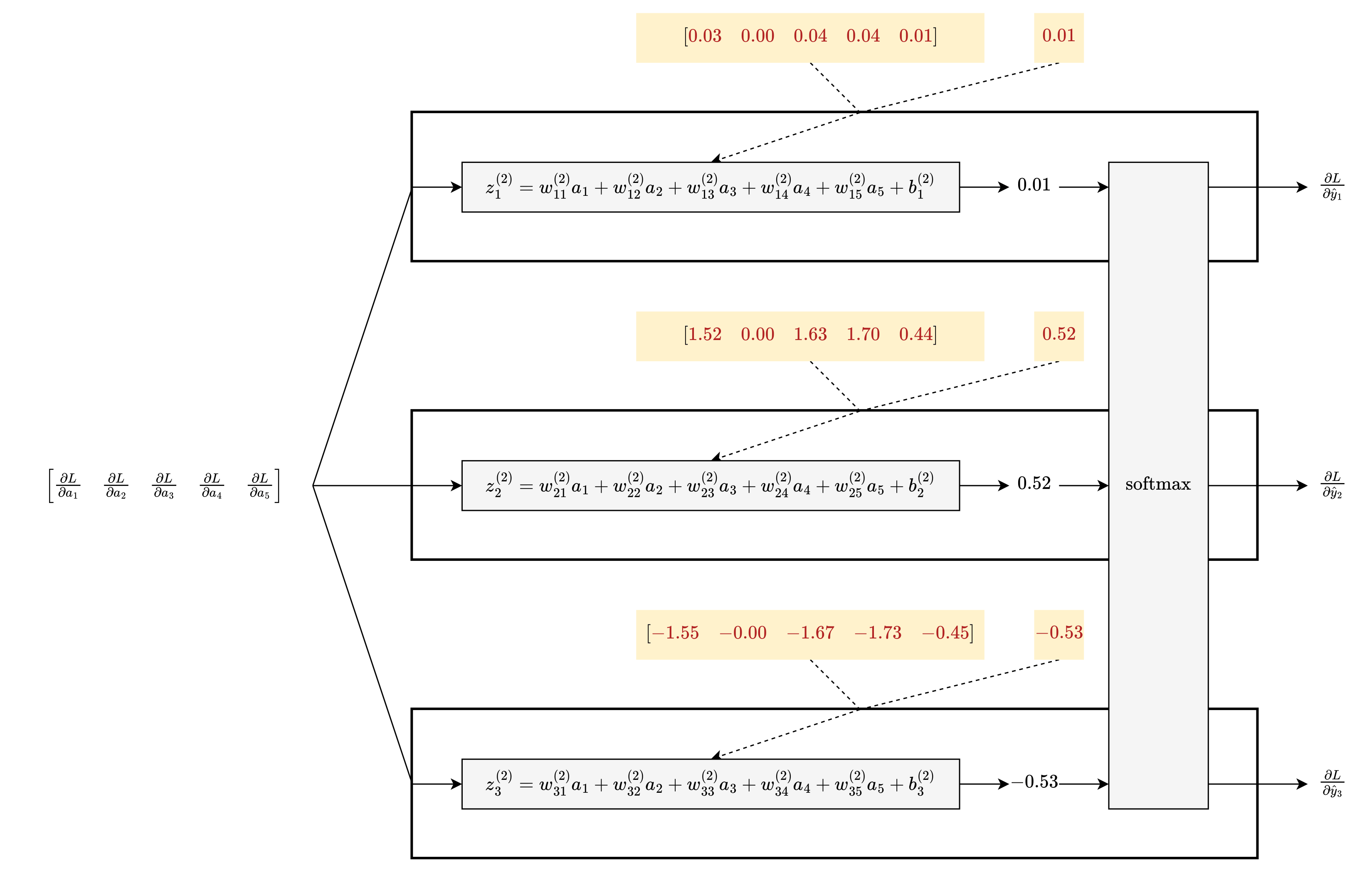
To calculate ∂L/∂a₁, however, you must take 3 steps:
During the forward pass, you fed a₁ forward to 3 functions.
During the backward pass, you must travel backward through all 3 functions.
The chain rule takes a different form here; it combines those 3 steps into 1 value:
Let’s walk through those 3 steps:
To create 3 backward links, convert 3 functions to 3 derivatives:
Functions:
\(\begin{bmatrix} z^{(2)}_1 \\ z^{(2)}_2 \\ z^{(2)}_3 \end{bmatrix} = \begin{bmatrix} w^{(2)}_{11} a_1 + w^{(2)}_{12} a_2 + w^{(2)}_{13} a_3 + w^{(2)}_{14} a_4 + w^{(2)}_{15} a_5 + b^{(2)}_1 \\ w^{(2)}_{21} a_1 + w^{(2)}_{22} a_2 + w^{(2)}_{23} a_3 + w^{(2)}_{24} a_4 + w^{(2)}_{25} a_5 + b^{(2)}_2 \\ w^{(2)}_{31} a_1 + w^{(2)}_{32} a_2 + w^{(2)}_{33} a_3 + w^{(2)}_{34} a_4 + w^{(2)}_{35} a_5 + b^{(2)}_3 \end{bmatrix}\)Derivatives:
\(\begin{bmatrix} \frac{\partial z^{(2)}_1}{\partial a_1} \\ \frac{\partial z^{(2)}_2}{\partial a_1} \\ \frac{\partial z^{(2)}_3}{\partial a_1} \end{bmatrix} = \begin{bmatrix} w^{(2)}_{11} \\ w^{(2)}_{21} \\ w^{(2)}_{31} \end{bmatrix}\)Retrieve the values from the forward pass:
\(\begin{bmatrix} \frac{\partial z^{(2)}_1}{\partial a_1} \\ \frac{\partial z^{(2)}_2}{\partial a_1} \\ \frac{\partial z^{(2)}_3}{\partial a_1} \end{bmatrix} = \begin{bmatrix} w^{(2)}_{11} \\ w^{(2)}_{21} \\ w^{(2)}_{31} \end{bmatrix} \approx \begin{bmatrix} -0.21 \\ 0.40 \\ 0.28 \end{bmatrix}\)
To use those 3 backward links, use the chain rule:
\(\begin{alignat*}{3} \frac{\partial L}{\partial a_1} &= \frac{\partial L}{\partial z^{(2)}_1} \frac{\partial z^{(2)}_1}{\partial a_1} &&+ \frac{\partial L}{\partial z^{(2)}_2} \frac{\partial z^{(2)}_2}{\partial a_1} &&+ \frac{\partial L}{\partial z^{(2)}_3} \frac{\partial z^{(2)}_3}{\partial a_1} \\ &\approx 0.01 \cdot -0.21 &&+ 0.52 \cdot 0.40 &&+ -0.53 \cdot 0.28 \\ &\approx 0.06 \end{alignat*}\)
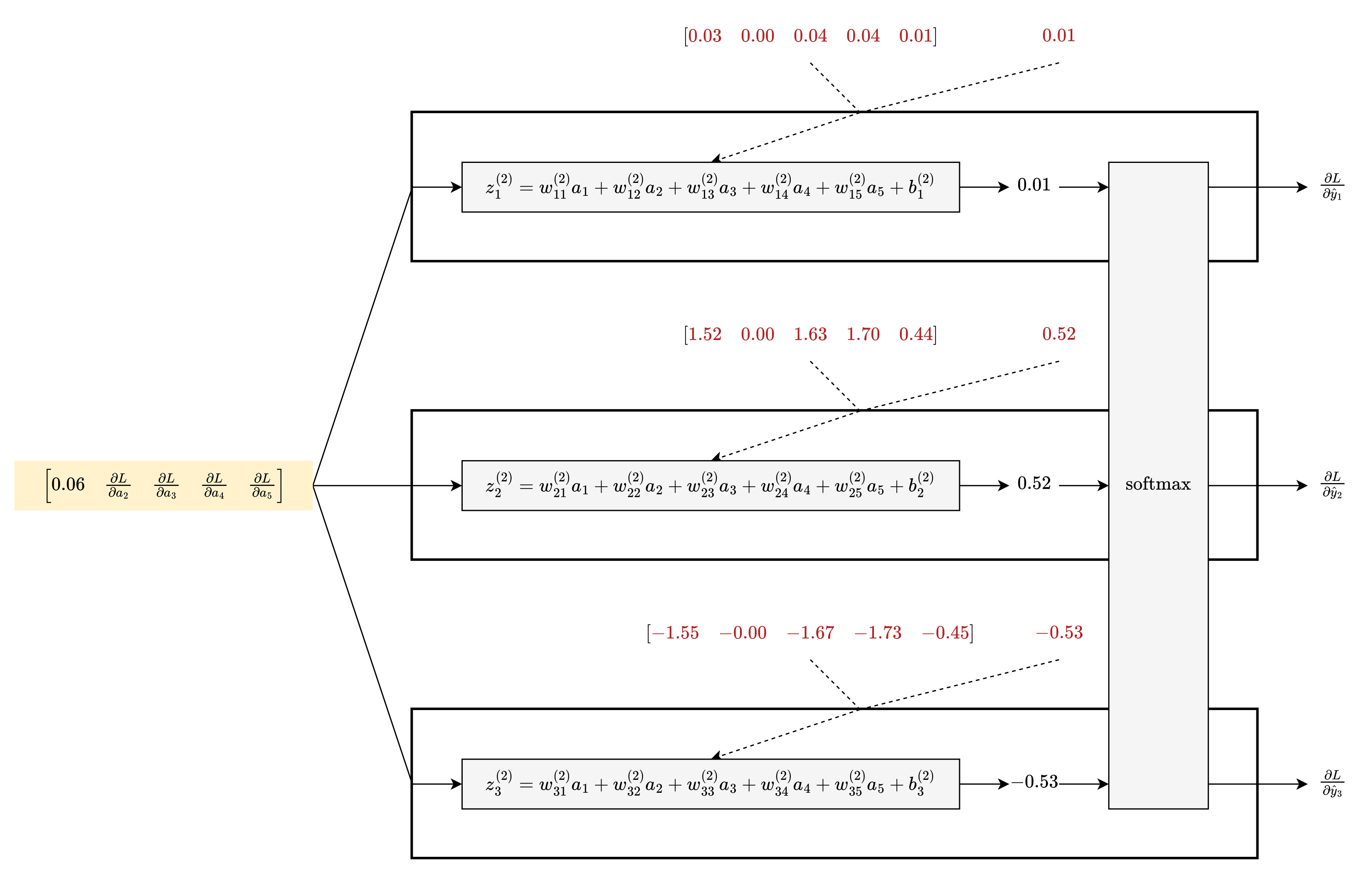
In a similar vein, you can take 12 more steps from the 3 logits to the other 4 a’s:
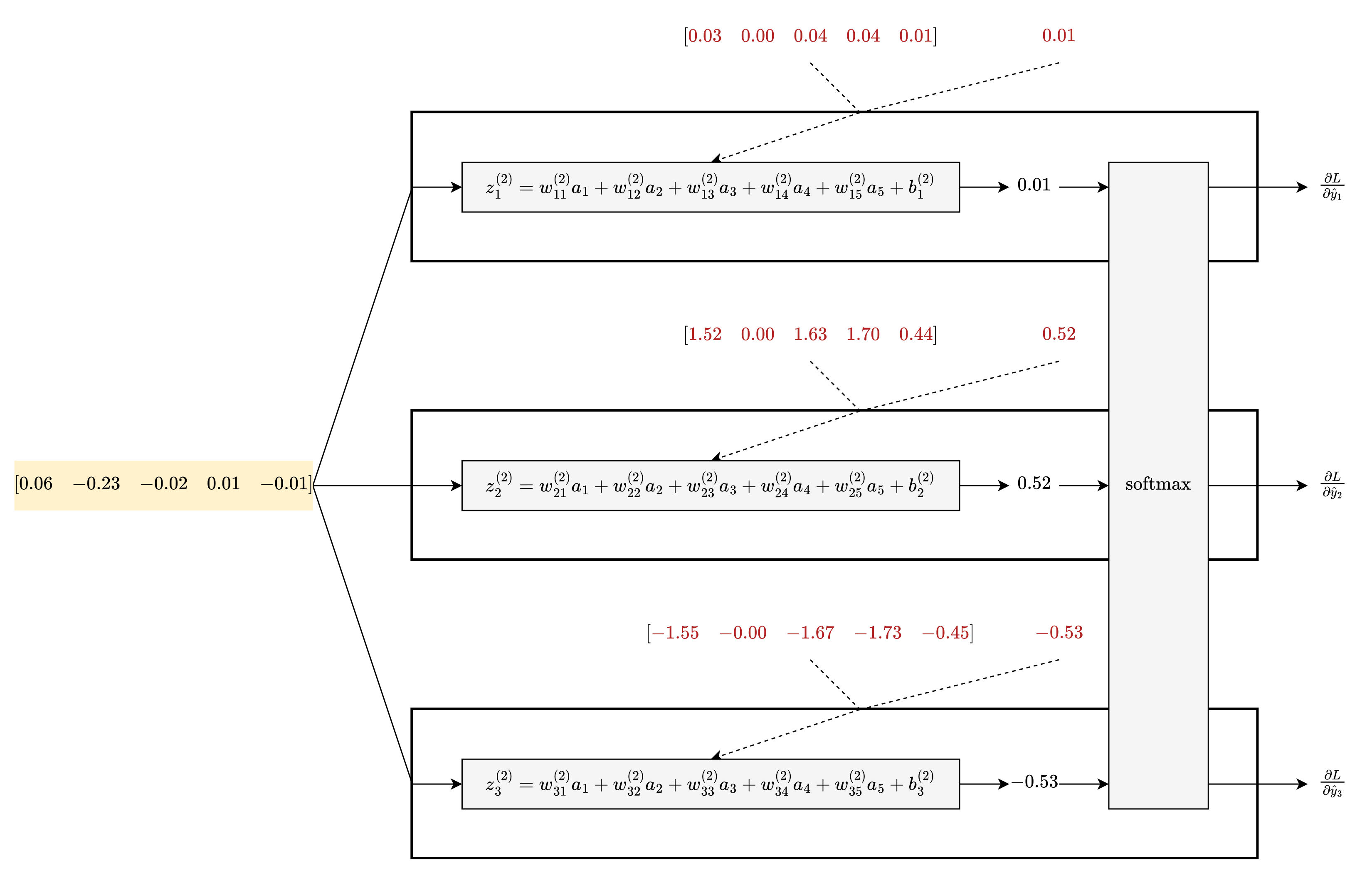
Once you reach the hidden layer, backpropagation works the same as before.
Learn
This video shows what happens when you train this neural network for 3000 steps:
Here are the trained parameters:
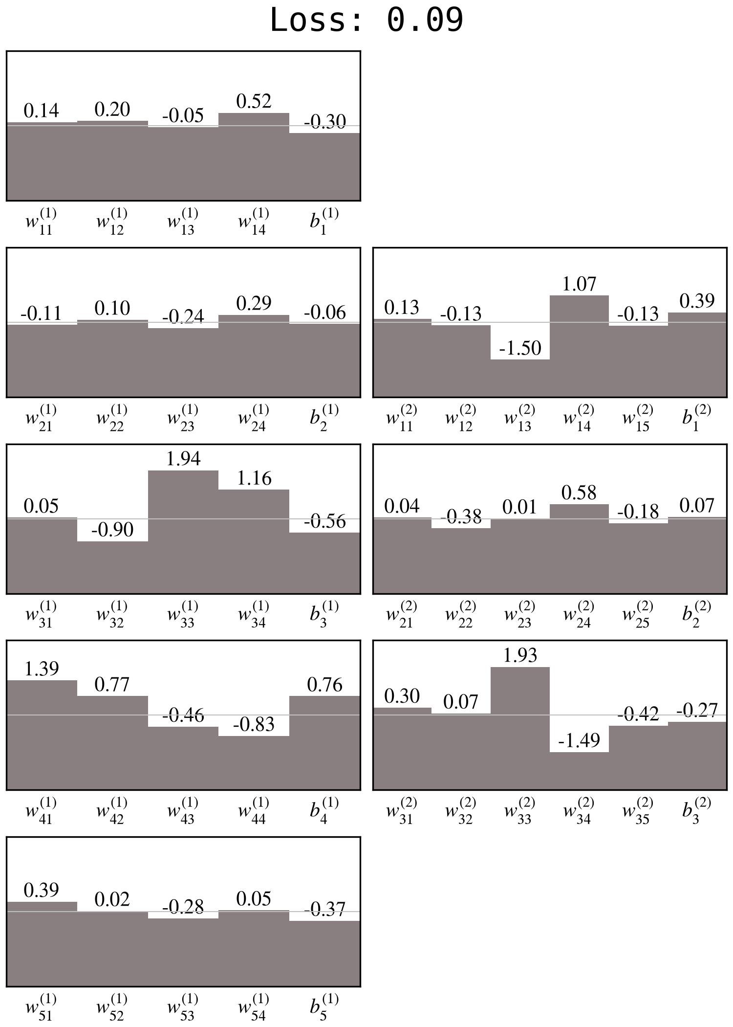
With trained parameters, here is the accuracy of the neural network:
For your sample, it correctly chooses iris virginica. Here are the probabilities:
iris setosa: nearly 0%
iris versicolor: approximately 4%
iris virginica: approximately 96%
For the training data, the accuracy is approximately 98.33% (118/120 samples).
For the test data, the accuracy is 100% (30/30 samples).
Test accuracy is the metric that matters.